Tools for Model Building and Good Practices¶

This section discusses the specific tools for recommended for building valid and robust statistical models. The RooFit pacakge is core to data modeling in ROOT.

We begin with a discussion of the RooFit philosophy - we want a single language for all measurements: common tools & joint model building (other tools) followed by a description of the RooFit language basics, and the workspace. A series of tools for building & manipulating models built using RooFit as a foundation are described with some links and general usage. Finally a list of good practices are presented regarding issues such as modeling systematics, uncertainties, and model cleaning among others.

RooFit¶

RooFit - a model building language¶

The main feature of the design of the RooFit/RooStats suite of statistical analysis tools is that the tools to build statistical models and the tools to perform statistical inference are separate, but interoperable. This interoperability is universally possible because all statistical inference is based on the likelihood function.

The goal is that all tools in the RooStats suite can analyse any model built in RooFit. The interoperability is facilitated in practice by the concept of the workspace (RooFit class RooWorkspace) that allows to persist statistical models of arbitrary complexity into ROOT files and thus allow to separate the model building phase and the statistical inference phase of a data analysis project both in space and time

RooFit basics¶

This section will cover the essentials of the RooFit modelling language, which wil aid in the understanding of the role of higher level modelling tools and model manipulation.

The key concept of RooFit probability models is that all components that form the mathematical expression of a probability model or probability density function are expressed in separate C++ objects. Base classes exist to represent e.g. variables, functions, normalised probability density functions, integrals of function, datasets, and implementations of many concrete functions and probability density functions are provided.

The examples below show how a Gaussian and Poisson probability model are built by constructing first the component objects (the parameters and observables), and the the probability (density) functions.

// Construct a Gaussian probability density model
RooRealVar x("x","x",0,-10,10) ;
RooRealVar mean("mean","Mean of Gaussian",0,-10,10) ;
RooRealVar width("width","With of Gaussian",3,0.1,10) ;
RooGaussian g("g","Gaussian",x, mean,width) ;

// Construct a Poisson probability model
RooRealVar n("n","Observed event cont",0,0,100) ;
RooRealVar mu("mu","Expected event count",10,0,100) ;
RooPoisson p("p","Poisson",n, mu) ;

# Construct a Gaussian probability density model
x = ROOT.RooRealVar("x","x",0,-10,10)
mean = ROOT.RooRealVar("mean","Mean of Gaussian",0,-10,10)
width = ROOT.RooRealVar("width","With of Gaussian",3,0.1,10)
g = ROOT.RooGaussian("g","Gaussian",ROOT.RooArgSet(x), mean,width)

# Construct a Poisson probability model
n = ROOT.RooRealVar("n","Observed event cont",0,0,100)
mu = ROOT.RooRealVar("mu","Expected event count",10,0,100)
p = ROOT.RooPoisson("p","Poisson",n, mu)

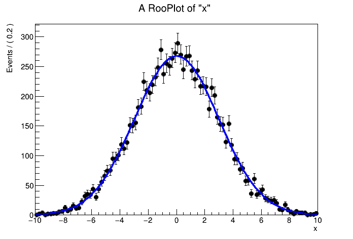
RooFit implements all basic functionality of statistical models: toy data generation, plotting, and fitting (interfacing ROOTs minimisers for the actual -logL minimisation process).

// generate unbnined dataset of 10k events
RooDataSet* toyData = g.generate(x,10000) ;

// Perform unbinned ML fit to toy data
g.fitTo(*toyData) ;

// Plot toy data and pdf in observable x
RooPlot* frame = x.frame() ;
toyData->plotOn(frame) ;
g.plotOn(frame) ;
frame->Draw() ;

# generate unbnined dataset of 10k events
toyData = g.generate(ROOT.RooArgSet(x),10000)

# Perform unbinned ML fit to toy data
g.fitTo(toyData)

# Plot toy data and pdf in observable x
frame = x.frame()
toyData.plotOn(frame)
g.plotOn(frame)
frame.Draw()

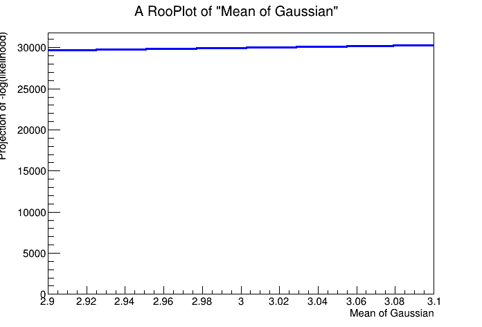
As the likelihood function plays an important role in many statistical techniques, it can also be explicitly constructed as a RooFit function object for more detailed control

// Create Likelihood function L(x|mu,sigma) for all x in toy data
RooAbsReal* nll = g.createNLL(*toyData) ;

// ML estimation of model parameters mean,width
RooMinimizer m(*nll) ;
m.migrad() ; // Minimization
m.hesse() ; // Hessian error analysis

// Result of minimisation and error analysis is propagated
// to variable objects representing model parameters
mean.Print() ;
width.Print() ;

// Visualize likelihood L(mu, sigma)
// at sigma = sigma_hat in range 2.9<mu<3.1
RooPlot* frame2 = mean.frame(2.9,3.1) ;
nll->plotOn(frame2) ;
frame2->Draw() ;

# Create Likelihood function L(x|mu,sigma) for all x in toy data
nll = g.createNLL(toyData)

# ML estimation of model parameters mean,width
m = ROOT.RooMinimizer(nll)
m.migrad()  # Minimization
m.hesse()   # Hessian error analysis

# Result of minimisation and error analysis is propagated
# to variable objects representing model parameters
mean.Print()
width.Print()

# Visualize likelihood L(mu, sigma)
# at sigma = sigma_hat in range 2.9<mu<3.1
frame2 = mean.frame(2.9,3.1)
nll.plotOn(frame2)
frame2.Draw()

RooFit implements a very wide range of options to tailor models and their use that are not discussed here in the interest of brevity, but are discussed in detail here <insert_link>. RooFit also automatically performs an optimisation of the computation strategy of each likelihood before each use, so that users that build models generally do not need to worry about specific performance considerations when expression the model. Example optimisations include automatic detection of unused dataset variables in a likelihood, automatic detection of expression that only depend on (presently) constant parameters and caching and lazy evaluation of expensive objects such as numerical integrals. The following links provide further information on a number of RooFit related topics

Guide to the RooFit workspace and factory language <LINK>
Guide to (automatic) computational optimizations in RooFit <LINK>
Guide to writing your own RooFit PDF classes <LINK>

RooFit workspace essentials¶

The key to the RooFit/RooStats approach of separating model building and statistical inference is the ability to persist built models into ROOT files and the ability to revive these with minimal effort in a later ROOT session. This ability is powered by the RooFit workspace class, in which built models can be important, which organises the persistence of these models, regardless of their complexity

 // Saving a model to the workspace
RooWorkspace w("w") ;
w.import(g) ;
w.import(p) ;
w.import(*toyData,RooFit::Rename("toyData")) ;
w.Print() ;
w.writeToFile("model.root") ;

// ————————————————

// Reviving a model from a workspace
TFile* f = TFile::Open("model.root") ;
RooWorkspace * w = (RooWorkspace*) f->Get("w") ;
RooAbsPdf* g = w->pdf("g") ;
RooAbsPdf* p = w->pdf("p") ;
RooDataSet* toyDatata = w->data("toyData") ;

# Saving a model to the workspace
w = ROOT.RooWorkspace("w")
getattr(w,'import')(g)
getattr(w,'import')(p)
getattr(w,'import')(toyData,ROOT.RooFit.Rename("toyData"))
w.Print()
w.writeToFile("model.root")

# ————————————————

# Reviving a model from a workspace
f = ROOT.TFile.Open("model.root")
w = f.Get("w")
g = w.pdf("g")
p = w.pdf("p")
toyDatata = w.data("toyData")

The code example above, while straightforward highlights a couple of important points

Reviving a model or dataset is always trivial, typically 3-4 lines of code depending on the number of objects that must be retrieved from the workspace, even for large workspaces e.g. full Higgs combinations that can contain over ten thousand component objects.
Retrieval of objects (functions, datasets) is indexed by their internal object, as giving to them in the first C++ constructor argument (all RooFit object inherit from ROOT class TNamed, which identical behaviour).
For objects where the model building user did not explicitly specify the objects intrinsic name, like the toyData object in the example above, it is possible to rename the object to a given name after the fact. The most convenient path to do this is to do this upon import in the workspace, as shown in the code example above.

The ModelConfig interface object¶

Since model and data names do not need to conform to any specific convention, the automatic operation of statistical tools in RooStats need some guidance from the user to point the tool the correct model and dataset. The interface between RooFit probability models and RooStats tools is the RooStats::ModelConfig object. The ModelConfig object has two clarifying roles

1. Identifying which pdf in the workspace is to be used for the calculation. The workspace content does not need to follow any particular naming convention. The ModelConfig object will guide the calculator the desired model

Specifying information on the statistical inference problem that is not intrinsic to the probability model:

i.e. which parameters are “of interest”, which ones are “nuisance”, what are the observables to be considered,

and (often) a set of parameter values that fully define a specific hypothesis (e.g. the null or alternate hypothesis)

Here is a code example that construct a ModelConfig for the Poisson probability model created earlier

// Create an empty ModelConfig
RooStats::ModelConfig mc("ModelConfig",&w);

// Define the pdf, the parameter of interest and the observables
mc.SetPdf(*w.pdf("p"));
mc.SetParametersOfInterest(*w.var("mu"));
mc.SetObservables(*w.var("n"));

// Define the value mu=1 as
// a fully-specified hypothesis to be tested later
w->var("mu")->setVal(1) ;
mc.SetSnapshot(*w.var("mu"));

// import model in the workspace
w.import(mc);

# Create an empty ModelConfig
mc = ROOT.RooStats.ModelConfig("ModelConfig",w)

# Define the pdf, the parameter of interest and the observables
mc.SetPdf(w.pdf("p"))
mc.SetParametersOfInterest(w.var("mu"))
mc.SetObservables(w.var("n"))

# Define the value mu=1 as
# a fully-specified hypothesis to be tested later
w.var("mu").setVal(1)
mc.SetSnapshot(*w.var("mu"))

# import model in the workspace
getattr(w,'import')(mc)

When the intent is to use RooStats tools on a model, it is common practice to insert a ModelConfig in the workspace in the model building phase so that the persistent workspace is fully self-guiding when the RooStats tools are run. More details on this are given in Section 4 on statistical inference tools. The presence of a ModelConfig object can of course also used to simply the use of workspace files outside the RooStats tools.

For example the code fragment below will perform a maximum likelihood fit on any workspace with a model and dataset and valid ModelConfig object

void run_fit(const char* workspaceName, const char* datasetName) {

    // Reviving a model from a workspace
    TFile* f = TFile::Open("model.root") ;
    RooWorkspace* w = (RooWorkspace*) f->Get("w") ;
    RooStats:::ModelConfig* mc = (RooStats::ModelConfig*) w->genobj("ModelConfig") ;
    RooAbsPdf* pdf = w->pdf(mc->GetPdf()->GetName()) ;

    // Load data from workspace
    RooAbsData* data = w->data(datasetName) ;

    if (!pdf || !data) return ;
    pdf->fitTo(*data) ;
}

def run_fit(workspaceName, datasetName):

    # Reviving a model from a workspace
    f = ROOT.TFile.Open("model.root")
    w = f.Get(workspaceName)
    mc = w.genobj("ModelConfig")
    pdf = w.pdf(mc.GetPdf().GetName())

    # Load data from workspace
    data = w.data(datasetName)

    if pdf is None or data is None: return None
    pdf.fitTo(data)

The example above is not completely universal, because it does not deal with ‘global observables’, this issue is explained further in later sections.

The workspace factory¶

To simplify the logistical process of building RooFit models, the workspace is also interfaced to a factory method that allows to fill a workspace with objects with a shorthand notation. A short description of the factory language is given here with the goal to be able to understand code examples given later in this section. A full description of the language is, along with a comprehensive description of other features of the workspace is given here <INSERT_LINK>

The workspace factory is invoked by calling the factory() method of the workspace and passing a string with a construction specification, which typically look like this:

RooWorkspace w("w") ;
w.factory("Gaussian::g(x[-10,10],m[0,-10,10],s[3,0.1,10])") ;
w.factory("Poisson::p(n[0,100],mu[3,0,100])") ;

RooWorkspace w("w")
w.factory("Gaussian::g(x[-10,10],m[0,-10,10],s[3,0.1,10])")
w.factory("Poisson::p(n[0,100],mu[3,0,100])") ;

The syntax of the factory, as shown, is simple because it is limited - the two essential operations are 1) creation of variable objects and 2) the creation of (probability) functions.

For the first task, the following set of expressions exist to create variables:

name[xmin,xmax] creates a variable with given name and range. The initial value is the middle of the range
name[value, xmin,xmax] creates a variable with given name and range and initial value
name[value] creates a named parameter with constant value
value creates an unnamed (and immutable) constant-value object
name[label,label,…] creates a discrete-valued variable (similar to a C++ enum) with a finite set of named states

For the second task, a single syntax exists to instantiate all RooFit pdf and function classes

ClassName::objectname(…) creates an instance of ClassName with the given object name (and identical title).

The three important rules are

The class must be known to ROOT (i.e. if it is defined in a shared library, it must have been loaded already). The prefix “Roo” of any class name can optionally be omitted for brevity
The meaning of the arguments supplied in the parentheses map to the constructor arguments of that class that follow after the name and title. In case multiple constructors exist in a class, they are tried in the order in which they are specified in the header file of the class.
Any argument that is specified must map to the name of an object that already exists in the workspace, or be created on the fly.

These factory language rules can be used to create objects one at a time, as is shown here

// Create empty workspace
RooWorkspace w("w") ;

// Create 3 variable objects -
//      to be used as observable and parameters of
//      a Gaussian probability density model
w.factory("x[-10,10]") ;
w.factory("mx[0,-10,10]") ;
w.factory("sx[3,0.1,10])") ;

// Create a Gaussian model using the previously defined variables
w.factory("Gaussian::sigx(x,mx,sx)") ;

// Print workspace contents
w.Print("t") ;

# Create empty workspace
w = ROOT.RooWorkspace("w")

# Create 3 variable objects -
#      to be used as observable and parameters of
#      a Gaussian probability density model
w.factory("x[-10,10]")
w.factory("mx[0,-10,10]")
w.factory("sx[3,0.1,10])")

# Create a Gaussian model using the previously defined variables
w.factory("Gaussian::sigx(x,mx,sx)")

# Print workspace contents
w.Print("t")

RooWorkspace(w) w contents

variables
---------
(mx,sx,x)

p.d.f.s
-------
RooGaussian::sig[ x=x mean=mx sigma=sx ] = 1

Creating models one object at a time, can still be quite space consuming, hence it possible to nest construction operations. Specifically, any syntax token that generates an object returns (e.g. x[-10,10]’) the name of the object created (‘x’) , so that it can be used immediately in an enclosing syntax token. Thus a nested construction specification can construct a composite object in a single token in a natural looking form. The four lines of factory code of the previous example can be contracted as follows

// Create a Gaussian model and all its variables
w.factory("Gaussian::sigx(x[-10,10],m[0,-10,10],s[3,0.1,10])") ;

Use of existing objects and newly created object can be freely mixed in any expression. The example below creates a second model for observable y using the same (existing) parameter objects as the Gaussian pdf sig:

// Create a Gaussian model using the previously defined parameters m,s
w.factory("Gaussian::sigy(y[-10,10],m,s)") ;

As the power of RooFit building lies in the ability combine existing pdfs, operator pdfs that multiply, add, or convolve components pdfs are frequently used. To simply their use in the factory, most RooFit-provided operator classes provide a custom syntax to the factory that is more intuitive to use than the constructor form of these operator classes. For example:

SUM::sum(fraction*model1,model2) - Sum two or more pdfs with given relative fraction.
PROD::product(modelx,modely) - Multiply two uncorrelated pdfs F(x) and G(y) of observables (x,y) in the same dataset into a joint distribution FG(x,y) = F(x)*G(y)
SIMUL::simpdf(index[SIG,CTL],SIG=sigModel,CTL=ctlModel) - Construct a joint model for to disjoint datasets that are described by distributions sigModel and ctlModel respectively
expr::func(’sin(a*x)+b’,a[-10,10],x,b[-10,10]) - Construct an interpreted RooFit function ‘func’ on the fly with the given formula expression.

The syntax for operators is not native to the language, but is part of the operator class definition, which can register custom construction expression with the factory. It is thus explicitly possible for all RooFit pdfs (both for operator and basic pdfs) to introduce additional syntax to the factory language A comprehensive list of the operator expression of all classes in the standard ROOT distribution of root is given here <INSERT_LINK>.

A complete example illustrate how the various language features work together to build a two-dimensional probability model with a signal and background component

A couple of final important points on RooFit models and workspace

The factory is an efficient way to quickly express what RooFit objects should be instantiated. Objects built with the factory

are not in any way different from those created ‘manually’ and then imported into the workspace.

All objects (wether created through the factory or imported) can be modified a posteriori, e.g. modification of advanced

settings from class methods, after they have been created and/or imported. All such changes in settings are persisted with the workspace. The factory does therefore on purpose not provide an interface for such modifications.

All RooFit objects in a workspace should have unique names. The factory and import methods automatically enforce this

Building joint models and data structures¶

the general case¶

When building joint probability models for multiple datasets, e.g. simultaneous fits or profile likelihood models in general, there are some important point to consider when building the model. In the RooFit paradigm such joint fits are best constructed by first joining all independent datasets together into a single composite ‘master’ dataset, and by joining all probability models corresponding to the individual datasets into a composite ‘master’ probability model. If it is done this way, all main statistical operations ranging from basic operations like fitting and toy data generation to advanced limit setting procedures work on composite models with exactly the same interface as for simple models. This design choices greatly simplifies the syntax of the high level statistical tools, but introduces some additional syntax to express composite datasets and probability models, which are discussion in this section.

Joining probability models for disjoint datasets

A joint probability model that simultaneously describes two or more disjoint datasets is represented in RooFit by class RooSimultaneous, which is constructed in the factory with the SIMUL operator:

// Construct joint model for signal region and a control region
// This example assumes a pdf sigModel and ctlModel were previously defined
// in the workspace (the internal structure of these models is irrelevant)
//
w.factory("SIMUL::master(index[SIG,CTL],SIG=sigModel,CTL=ctlModel)") ;

The code above generates two new objects

A new discrete observable (class RooCategory) named ‘index’ that has two defined states: SIG and CTL that serves

as additional observable to the newly create pdf master (in addition to the observables defined in sigModel and ctlModel). The role of this observable is to indicate which component pdf should be used to interpret the remaining observables in the dataset

A new joint probability model master that describes both distributions. Suppose sigModel describes the distribution

of observable x and ctlModel describes the distribution of observable y, then the observables of the joint model are {index, x, y}

Joining disjoint datasets into a master dataset

The joint dataset that is needed to construct a likelihood from ‘master’ model must thus also conform to this structure: it’s observable must include both x and y, as well as the discrete index variable to label to which component dataset each event belongs. It is instructive to first consider visually what this data organization entails

D(x)    D(y)       D(index,x,y)
1.5     23           SIG, 1.5, -
2.3     17    —>     SIG, 2.3, -
4.7     98           SIG, 4.7, -
                     CTL,  - , 23
                     CTL,  - , 17
                     CTL,  - , 98

The joining of datasets is trivially perform in the RooDataSet constructor

// The example assume this existence of a workspace that defines variable, x,y,index

// Construct a dataset D(x)
RooDataSet d_sig("d_sig","d_sig",*w.var("x")) ;
w.var("x")->setValue(1.5) ;
d_sig.add(*w.var("x")) ; // fill data, etc..

// Construct a dataset D(y)
RooDataSet d_ctl("d_ctl","d_ctl",*w.var("y")) ;
w.var("y")->setValue(23) ;
d_ctl.add(*w.var("xy")) ; // fill data, etc..

// Construct a joint dataset D(index,x,y)
map<string,RooDataSet*> dmap;
dmap["SIG"]=&d_sig ;
dmap["CTL"]=&d_ctl ;

RooDataSet d_joint("d_joint","d_joint",Index(*w.cat("index")),Import(dmap)) ;

Note that while a composite RooDataSet externally presents the interface of a simple dataset with observables (index,x,y) it is internally organised in subdatasets for efficient storage and data retrieval

D(index,x,y)           D(index,x,y)
SIG, 1.5, -               index==SIG     index==CTL
SIG, 2.3, -                 D(x)            D(y)
SIG, 4.7, -       —>        1.5             23
CTL,  - , 23                2.3             17
CTL,  - , 17                4.7             98
CTL,  - , 98

This internal data organization is also introduced for toy data sets that are sampled from composite datasets.

Working with joint models and datasets

Once the joint model master(index,x,y) and a joint dataset D(index,x,y) are constructed, all operations work exactly as for simple models. For example, a joint fit is trivially performed as follows

w.pdf("master")->fitTo(d_joint) ;

An important part of the design of joint models is that there is no performance loss due to computation overhead in the joint construction: when the joint likelihood is constructed from a joint model and dataset, it is internally organised again in component likelihoods, where each component model of master is match to the corresponding component dataset of d_joint, and subsequently separately optimised for computational efficiency.

profile likelihood models & global observables¶

While the interface described in the previous sections works for joint models of any shape and form, a dedicated syntax exists for the formulation of so-called ‘profile likelihood’ models. The key difference between a generic joint model and a ‘profile likelihood’ joint model is that in the latter the internal structure of the control region (now named ‘subsidiary measurement’ is simplified to a Gaussian, Poisson or LogNormal distribution so that the corresponding observation can be represented by a single number, where the convention of the subsidiary measurement is furthermore chosen such, through a suitable transformation of the meaning of the parameters, that the observed values is either always zero or one

\[\mathcal{L}_\mathrm{joint}(p,q) = \mathcal{L}_\mathrm{sig}(x_\mathrm{sig} | \mu, \theta) * \mathcal{L}_\mathrm{ctl}( y_\mathrm{ctl} | \theta )\]

\[\Downarrow\]

\[\mathcal{L}_\mathrm{profile} ( \mu, \alpha) = \mathcal{L}_\mathrm{sig} (x_\mathrm{sig} | \mu, \alpha) * \mathcal{L}_\mathrm{subs}( 0 | \alpha)\]

Such likelihood can in principle be described with a joint dataset \(D`(index,:math:`x_\mathrm{sig}\),0,0,….0) and a corresponding SIMUL probability model with equally many components, but the carrying around of hundreds of observed values that are always identical to zero can be cumbersome.

Hence an alternative formulation style exists in RooFit that is specifically suitable for profile likelihood models - here the observed value of the subsidiary measurements is simply encoded in observable variable of the pdf itself, rather than in an external dataset. Hence instead of a dataset/model pair in traditional joint format

\[\mathcal{D}_\mathrm{simul}(\mathrm{index},x_\mathrm{sig},y_\mathrm{ctl}==0)\]

\[\mathrm{and}\]

\[\mathrm{pdf}_\mathrm{simul}(\mathrm{index},x_\mathrm{sig},y_\mathrm{ctl} | \mu, \alpha) = \mathrm{pdf}_\mathrm{sig}(x_\mathrm{sig}|\mu,\alpha) * \mathrm{pdf}_\mathrm{subs}(y_\mathrm{ctl}|\alpha)\]

one writes

\[\mathcal{D}_\mathrm{simul}(x_\mathrm{sig})\]

\[\mathrm{and}\]

\[\mathrm{pdf}_\mathrm{simul}(x_\mathrm{sig},y_\mathrm{ctl}==0 | \mu, \alpha) = \mathrm{pdf}_\mathrm{sig}(x_\mathrm{sig}|\mu,\alpha) * \mathrm{pdf}_\mathrm{subs}(0|\alpha)\]

where the observable \(y_\mathrm{ctl}==0\) is dropped from the dataset, as well as the index observable, as it is no longer needed to distinguish between data belonging to the main measurement and the subsidiary measurement(s). This greatly simplifies the formulation of datasets of profile likelihood models. On the probability model side, the formulation then changes as follows

Instead of using SIMUL() to multiply subsidiary measurements with the main measurement, the PROD() operator

is used, which does not require the introduction of an index observable to label events

The model variables that represent the subsidiary measurements must be explicitly labeled in the object as such

(to distinguish these from parameters). This can be either done intrinsically in the model, or this specification can be provided externally when an operation (fit, toyMC generation etc) is performed

In the LHC jargon the variables in the model that represent the (trivial) values of the observables of the subsidiary measurements are named the “Global Observables”. The easiest-to-use way to mark global observables in the model is to label them as such

// repeat for each global observable
w.var(“obs_alpha”)->setAttribute(“MyGlobalObservable”) ;

// advertise string label used to mark global observables in the top-level pdf object
w.pdf(“master”)->setStringAttribute(“GlobalObservablesTag”,”MyGlobalObservable”) ;

Most modeling building tools currently in use, do not yet take advantage to label these observables as such in the model. Instead it is common practice, to specify these always external through a GlobalObservables() command-line specification when fitting or generation. To simplify this external specification process for RooStats tools, the ModelConfig interface object allows the global observables to be specified there, so that its definition is always consistently used by all RooStats tools.

 // Define the pdf, the parameter of interest and the observables
mc.SetPdf(*w.pdf(“p"));
mc.SetParametersOfInterest(*w.var("mu"));
mc.SetGlobalObservables(…..);
mc.SetObservables(*w.var(“n"));

Any code that works with profile likelihood that wishes this external specification of the global observables, in addition to the internal specifications must incorporate some explicit handling of thus. Here is a modified version of the run_fit() macro of the previous section that does so

void run_fit(const char* workspaceName, const char* datasetName) {

    // Reviving a model from a workspace
    TFile* f = TFile::Open("model.root") ;
    RooWorkspace* w = (RooWorkspace*) f->Get("w") ;
    RooStats:::ModelConfig* mc = (RooStats::ModelConfig*) w->genobj("ModelConfig") ;
    RooAbsPdf* pdf = w->pdf(mc->GetPdf()->GetName()) ;
    RooArgSet* globs = mc->GetGlobalObservables() ;

    // Load data from workspace
    RooAbsData* data = w->data(datasetName) ;

    if (!pdf || !data) return ;

    if (globs) {
            pdf->fitTo(*data, GlobalObservables(*globs)) ;
    } else {
      pdf->fitTo(*data)
}

def run_fit(workspaceName, datasetName):

    # Reviving a model from a workspace
    f = ROOT.TFile.Open("model.root")
    w = f.Get(workspaceName)
    mc = w.genobj("ModelConfig")
    pdf = w.pdf(mc.GetPdf().GetName())
    globs = mc.GetGlobalObservables()

    # Load data from workspace
    data = w.data(datasetName)

    if pdf is None or data is None: return None

    if globs:
      pdf.fitTo(data, ROOT.RooFit.GlobalObservables(globs))
    else:
      pdf.fitTo(data)

The processing of intrinsic global variable specifications is always automatic, but unfortunately it’s use is not common practice yet in LHC models.

Tools for model building and model manipulation¶

List of available tools [ Combiners, HistFactory, HistFitter, etc… ]

HistFactory

Improvements Needed/Planned¶

The core modeling framework of RooFit is quite mature, though a number of optimizations are still planned. In particular, for statistical models based on nominal and variational histograms, there is are challenges associated to the interpolation between histograms (including the ability to handle simultaneous variation of multiple nuisance parameters) and the handling of Monte Carlo statistical uncertainties in the histograms themselves (which are typically correlated in a non-trivial way among the variational histograms for a particular Monte Carlo sample). Work on these topics requires a careful dedicated effort, thus it is much more efficient if this effort is coordinated around a common code-base. The Statistics Forum has chosen to organize this effort with the goal of making a HistFactory v2.

There are a number of discussions about the tools being provided by the combined performance groups for evaluating systematics, these topics are outside of the scope of this document.

The issue of merging and “pruning” nuisance parameters from a model given the rapid growth of nuisance parameters we are currently experiencing. This is the topic for a separate document, and suggestions made are expected to propagate into the workplane the Statistics Forum is organizing for improvements to the modeling tools.

Good Practices¶

Good practices in model building¶

control and validation regions [ Exo ]

Modeling systematics - Correlations¶

Correlation modeling (prior and observed) [ Exo, Guide, some new material needed ]

Modeling systematic uncertainties - shape vs rate¶

[ Exo, WV slides ]

Modeling systematics - 2point discussion¶

[ Guide to PLL but needs updating ]

Modeling systematcs - pruning and smoothing¶

[ Exo ]

Modeling systematics - DOF¶

how many DOFs does your conceptual systematic have? [ Guide to PLL ]

Modeling uncertainties with increasing luminosity uncertainty¶

[ FAQ ]

Understanding computational aspects of the likelihood¶

Understanding computational performance¶

As probability models grow in complexity, the calculation time of likelihood functions can become a limiting factor. Models expressed in RooFit allow the RooFit core code complete introspection in the model structure and can automatically apply a series of performance optimizations to make calculations more effient and thus allow for faster calculations. Most of these techniques are applied automatically, few of them must be optionally activated. This section outlines the essence of optimization techniques that are applied and serves to further the understanding of model computation times in RooFit.

When are optimizations applied?

RooFit generally distinguishes two modes of operation - inside bulk operations (likelihood calculation, or toy event generation) and outside bulk operations. Most optimizations are applied inside the context of a bulk operation, where performance is more critical, and where more optimization opportunities exist as the use case of probability models is more clearly spelled out. Bulk operations in RooFit always operate on a clone of the original pdf, allowing to make non-resverrable use-case specific optimisation modifications to the model. The cloned model is discarded at the end of the bulk operation

Analytical integrals where possible

When RooFit is used to specify probability density functions (e.g. a Gaussian in a real-valued observable x) rather than as a probabillity model (e.g. a Poisson in a discrete-valued observable n), integrals must be explicitly calculated to make such probability density functions unit-normalized. As RooFit pdfs have no intrinsic convention of which of their variables are observables versus parameters, a calculation of a pdf as normalized probability density function must always be accompanied with a ‘normalization set’, which defines the subset of pdf variables that must be interpret as observables, and hence over which the expression must be normalized:

w.factory("Gaussian::g(x[-10,10],m[-10,10],s[3,0.1,10])") ;
RooArgSet normset(*w.var("x")) ;
Double_t g_normalized_wrt_x = w.pdf("g")->getVal(normSet) ; // calculate g as pdf for observable x

When called in this form, a separate RooFit object is created of class RooRealIntegral that represents the integral int_g(m,g) = Int g(x,m,g) dx over the defined range of variable x. RooFit function objects can advertise and implement (partial) analytical integrals in any (sub)set of their variables, for the cases where these expressions are analytically known. Whenever an integral over a pdf is needed in a likelihood evaluation (or other RooFit operation), the RooFit integral representation object RooRealIntegral will negotiate with the pdf if any suitable (partial) analytical integrals exists that match the requeste integration, and use those. Any remaining partial integrals that can not be integrated analytically, will be integrated numerically. When numerical integrals are used, information messages are emitted on the command line, and some user configuration/intervention may be needed to optimize performance (see section XXX on performance tuning for further details)

Integral representation objects that are used for pdf normalization purposes, as shown in the example above, are cached and owned by the pdf that requires them - hence the negotiated optimal calculation strategy is not redetermined at every call for a normalized pdf value, but kept for the lifetime of the pdf object, or until the pdf is structurally modified by the user in which case it is discarded and will be recreated on demand later if needed.

Change tracking and lazy evaluation (likelihood calculation & normal use)

The output value of each RooFit function object, as calculated by the classes implementation of method RooAbsReal::evaluate() is cached automatically in data member RooAbsReal::_value, when RooAbsReal::getVal() is called. A subsequent call to getVal() will simply return the previously calculated and cached value, unless it is detetermined that one or more of the inputs to the calculation has changed. RooFit tracks such changes through client-server links it maintains between all components of a pdf (whenever a dependent component of a RooFit function object is held in a data member of class RooRealProxy, RooListProxy or RooSetProxy, such links are automatically initiated). Each link (and each proxy) indicates if the object it is member of depends on the value or the shape of the server object. For real-valued objects, the shape of servers objects relates to the boundaries of the allowed values for that object.

For example, for a Gaussian pdf constructed as follows

w.factory("Gaussian::g(x[-10,10],m[-10,10],s[3,0.1,10])") ;

the object RooGaussian::g will consider the objects RooRealVar::x, RooRealVar::m and RooRealVar::m as it servers, and the latter 3 objects will consider RooGaussian::g as its client. When RooGaussian::g is constructed, it will indicate that it’s own value depends on the value of these three variables (but not on the shape). [ The configuration of this dependency information is encoded in the constructors of the proxy data members that hold x, m and g ]

The effect of that is that whenever one or more of the three variables changes its value, it will propagate a ‘value-changed’ message to all its clients (in this case RooGaussian::g), and this will set a ‘dirty’ flag on the value cache of that object. The raising of this dirty flag will not automatically trigger a recalculation of the value of g, but merely indicate that this must happen the next time g.getVal() is called, hence the name ‘lazy evaluation’.

Caching and lazy evaluation is of particular importance for normalization integrals: when the value of pdf g is requested as a normalized probability density function w.r.t to observable x, e.g.

RooArgSet normset(*w.var("x")) ;
Double_t g_normalized_wrt_x = w.pdf("g")->getVal(normSet) ;

a separate object is created that represents the integral Int g(x) dx, which depends on the values of parameters m and g, and the shape (range) of observable x, but not on the value of observable x.

When is caching and lazy evaluation applied?

Caching and lazy evaluation is active by default on all RooFit objects, whether directly created on the command line or in a workspace. Inside a likelihood function a slightly different strategy is applied - as a likelihood entails a series of pdf evaluation where the value of the observable changes (in principle) every time there is no point in tracking dependencies of direct or indirect pdf dependencies on dataset observables, as the result is such a check is already predetermined - each one will need to be recalculated for every consecutive event. Hence for all pdf and function components inside a likelihood that depend directly or indirectly on dataset observables, change tracking is disabled, to save the time that is spent in this unnecessary tracking. The notable exception to this are the normalization integral objects, which do not depend on the value of the dataset observables, but just on their range - these will remain in cache/lazy-eval mode inside likelihood objects, and thus only be recalculated on the less frequent occastion that one of the dependent model paremeters changes.

Constant term detection (likelihood calculation)

Certain parts of a probability model may depend only on parameter objects that are declared constant (RooRealVar::setConstant(kTRUE)). While the constant flag does not prevent manual modification of such a variable through a call to RooRealVar::setValue(), parameters that are flagged as constant will not be modified by the minimizer algorithm during a likelihood minimization are thus effectively constant during a minimization session. RooFit automatically detects all expressions in a likelihood that are effectively constant at the start of each minimization session and precalculates and caches their value along with the dataset. For example, for a composite pdf with signal and background

RooWorkspace w("w") ;
w.factory("SUM::model(fsig[0,1]*sig::Gausian(x[-10,10],m[-10,10],s[3]),bkg::Polynomial(x,{a0[0],a1[1]}))") ;

the background pdf bkg::Polynomial has only constant parameters (a0 and a1) hence its value is precalculated for every value of x in the dataset of a likelihood, and effectively added as a column to the internal dataset. A message to this effect is shown on the command line when the likelihood is initialized

When each event is loaded from the dataset in the likelihood calculation loop, the precalculated value of bkg::Polynomial is directly loaded in the value cache of that pdf, and it’s internal recalculation is skipped. Higher-level objects that depend on these cached elements, SUM::model in the example above, will then simply use the cached expression.

For pdfs expressions with multiple layers of composition operations, it is possible that entire trees of expression become constant. Consider for example

Here the background pdf is a sum of a general background and a peaking background that are first added together, before it is added to the signal. In this scenario, three pdf components in the full expression are constant: peakbkg, polybkg and sumbkg. In this particular scenario it is not needed to precalculate and cache all three pdfs: polybkg and sumbkg do not need to be cached separately as all of their clients (in this case just one - SUM::sumbkg) exclusively depend on constant expressions, hence they are never needed during the pdf evaluation - therefore only sumbkg is precalculated and cached, and peakbkg and polybkg are completely deactivated during the likelihood evaluation.

When is constant term optimization applied?

Constant term detection and precalculation only applies to likelihood calculations is automatically applied when RooAbsPdf::fitTo() is called. If you set up the minimization yourself, it must be explicitly activated manually when you configure the minimizer

RooAbsReal* nll = pdf->createNLL(*data,…) ;
RooMinimizer m(*nll) ;
m.optimizeConst(1) ; // This line activates constant term optimization
m.migrad() ;
m.hesse() ;
// etc

Cache-and-track optimization (likelihood calculation)

Cache-and-track optimization is an extension of the concept of constant-term optimization that can further reduce calculation times by exploiting typical likelihood usage patterns of minimization algorithms like MINUIT.

Apart from it’s setup phase, a likelihood minimization in Minuit(2) alternates two modes of operation: gradient calculations - where one parameter is changed per likelihood call - and gradient descent - where all parameters are changed for every likelihood call. For likelihoods with many parameters the gradient calculation calls dominate MINUITs likelihood evaluations as it requires N (parameter) calls to calculate the full gradient, whereas the gradient descent phase typically takes O(3) calls, independent of the number of parameters. If in the majority of likelihood calls from MINUIT only one parameter is changed, many component pdfs remain unchanged between likelihood calls, as typically a small subset of all pdf components will depend on the single parameter that changed.

In cache-and-track configuration, in addition to the truly constant terms, all component pdfs of a SUM and PROD composite models will be cached, as if they were constant, but a change tracker is included for these component that determines if the cache needs to be updated later (i.e. when a parameter of the pdf has changed w.r.t to the values that were used to calculate the cache contents). For the example pdf below, with only floating parameters in both signal (m) and background ( a0 , a1 )

RooWorkspace w("w") ;
w.factory("SUM::model(fsig[0,1]*sig::Gausian(x[-10,10],m[-10,10],s[3]),bkg::Polynomial(x,{a0[0,1],a1[0,1]}))") ;

both sig and bkg components can be cache-and-tracked, which has the following effect on the likelihood evaluation for the gradient calculation

gradient parameter	components cached	components recalculated
fsig m a0 a1	sig,bkg bkg sig sig	model sig,model bkg,model bkg,model

A clear saving is realized for the likelihood evaluations required for MINUITs gradient calculation, as only 1 or 2 of the 3 components pdfs need recalculation, instead of always all three of them, as would be required without cache-and-track.

When is cache-and-track optimization applied?

Cache-and-track optimization only applies to calculations within a likelihood. As the efficiency of cache-and-track optimization is highly dependent on the structure of the likelihood, it is not activated by default. To activate cache-and-track optimization of the likelihood, change the value of the argument to RooMinimizer::optimizeConst() from 1 to 2, or alternatively pass argument Optimize(2) to RooAbsPdf::fitTo().

Optimizing calculations with zero weights

In models that multiply pdf components (e.g. inside class PROD) it can happen that a product term evaluates to zero. If this occurs, the product calculation for that event is terminated immediately, and remaining product terms are no longer evaluated. Similarly, for weighted datasets (binned or unbinned), if the event weight is zero, the probability model for that event is not calculated.

When is zero-weight optimization applied?

Always automatically applied

Understanding issues with parallel calculation of likelihoods¶

The current RooFit version (v3.6x) has a simple built-in strategy to parallelize likelihood calculations over multiple cores on the same host, To activate this option, add the option NumCPU(n) to either RooAbsPdf::createNLL() or RooAbsPdf::fitTo(). It is important to understand the limitations of the paralellization algorithm:

The invocation of NumCPU(N) splits the workload of the likelihood (or each top-level likelihood object in case the top-level pdf is a SIMUL) in N equal sizes by dividing the number of data events offered to each of the N subprocesses in equal subsets. For unbinned datasets, the dataset is partitioned in N equal-size contiguous pieces. For binned datasets (i.e. histograms). the data is partitioned in equal sizes with an interleaving algorithm since histograms can be unevenly distributed. (Equal-size contiguous histogram partitions are prone to a substantial inbalance of partitions with zero event counts).

While the protocol overhead for parallelization is low, there are two major factors that spoil the scaling of wall-time speedup with the number of cores:

Expensive (numerical) integral calculations required in pdfs. Integral calculations are currently not distributed, but replicated among calculation threads.Hence if the total calculation time of a likelihood is dominated by (numerical) integrals, rather than PDF evaluations, wall-time gains realized by parallelization will be limited
Strongly heterogenous model structure. For wall-time scaling to be efficient, it is important that the workload can be divided in N partitions that each require the very similar, and ideally the exact same, calculation time. If the partitions end up not having very similar calculation times, the wall time will be dominated by the calculation time of the longest partition, which easily frustrates scaling beyond N =2,3. Models that are prone to load-imbalancing are those that have many binned dataset with variable and small sizes. For example the likelihood calculations based on histogram with 1 or 2 bins is not easily distributed in a balanced way over 4 CPUs.

In practice, all binned likelihoods built i ATLAS/CMS are strongly heterogeneous and thus poorly scalable. Unbinned ML fits, as typically executed in B-physics, are usually well-scalable. A new version of the RooFit parallel scheduler is being developed that addresses the load balancing issues with a dynamic scheduling polocy for strongly heterogenous pdfs, and is expected to be available late 2018, early 2019.

Also note that parallel calculated likelihood may return marginally different likelihood values, at the level of numeric precision of the calculation, as the order in which likelihood contributions from the data points are summed is inherently different. For marginally stable or unstable fit models, such small perturbations in the calculation may make the difference between convergence and failure, but it is important to diagnose this properly - the cause of the problem is the marginal stability, not the parallelized calculation.

Understanding the numeric precision and stability of calculations¶

In complex models it is not uncommon that limiting numeric precision becomes an issues and will lead to numerical instability of calculations. Numerical problems can have many causes, and can manifest themselves in many different forms. This section will focus only on issues arising from limited numeric precision arising in likelihood calculations, and not on issues arising from building models from poor information that are intrinsically well calculable but contain little useful information (e.g. template morphing models with low template statistics).

At what level of precision must the likelihood be calculable?

To understand when numeric precision in likelihood calculations becomes limiting it is important to understand how likelihoods are used by (minimization) tools. As most frequentist statistics tools boil down to minimization problems we will focus on what is needed for a stable minimization of a likelihood. At a fundamental level minimizers require that the likelihood, it’s first and second derivative are continuous. While most likelihoods meet these requirements at the conceptual level, numerical noise may spoil these features in their implementation. The most susceptible calculation of minimizers to noise is the numeric calculations of the first derivatives, evaluated as \(f(x) - f(x+\delta x)/\delta\), for comparively small values of \(\delta\). Jitter in the likelihood function, introduced by numerical noise, may thus result in wildly varying estimates of such derivatives when scanning over the parameters, if the frequency of the noise is comparable in size to \(\delta x\). In practice, an absolute precision at the level of 10 \(^{-6}\), is the barely tolerated maximum level of noise for minimizers like MINUIT, with target precisions at 10 \(^{-7}\) or 10 \(^{-8}\) often resulting in substantially faster converge and minimization stability.

Sources of numeric noise in the likelihood

There are two common source of noise in the likelihood: limited precision numeric integration of pdfs, and cumulative rounding/truncation effects of likelihoods.

Numeric integration noise

Numeric integration of functions is a notoriously hard computational problem, for which many algorithms exist. For reasons of speed and stability, analytical integrals are strongly preferred, and RooFit classes provide these when available. Nevertheless for many classes of functions no analytical expressions exist, and RooFit will substitute a numerical calculations. When considering numeric integrals, one-dimensional and multi-dimensional integrals represent challenges of a vastly different magnitude.

Numeric noise in 1-dimensional integrals.

Excellent numeric algorithms exist for one-dimensional integration that not only estimate the integral, but also its accuracy well, hence letting the (often iterative) integration algorithm reach the target precision for every integral in a reasonable amount of computing time. For well-behaved functions (i.e. no singularities or discontinuities) RooFits default algorithm, the adaptive Gauss-Kronrod integration, will rarely cause numeric problems with the default target precision of 10 \(^{-7}\) (considered both absolute and relative).

However, if the integrands are ill-suited, e.g. consider a histogram-shaped function with multiple discontinuities, integration algorithms can fail in various way: its error estimate may underestimate the true error, leading to larger variations of the calculated integral as function of the integrands parameter than the target tolerance, resulting in intolerable numeric noise in the likelihood. Alternatively, the algorithm may start ‘hunting’, switching forth and back between levels of iteration where it declares convergence at the requested level of precision, again as function of the integrands parameters, leading to spikes or jumps in the calculated integral. In particularly adaptive algorithms, that recursively subdivide the domain of the integral in smaller pieces, are susceptible to all of these failings with every additional subdivision. If the integrand is not pathological - the first defence against numeric instability from integrands is simply to increase the target precision. If that does not result in improvements and/or if the function has ‘difficult’ features, it may be advisable to try non-adaptive integration algorithms, which may require more function calls to converge, but are generally more stable in their result as function of the model parameters.

Numeric noise in multi-dimensional integrals.

Numeric integration in more than one dimension is notoriously hard, with an unfavorable tradeoff between computing time and numeric precision. The best solution is to avoid numeric multi-dimensional integration, by considering the feasibility of partial analytical integrals (RooFit explicitly supports hybrid analytical/numeric integrals in multiple dimensions). If this is not feasible, some careful tuning of algorithms is usually required, as multi-dimensional integrals rarely run at a satisfactory working point concerning speed and precision out of the box. For integrals of low dimensions (2,3), adaptive cubature integrals can be considered (the multidimensional equivalent of Gauss-Kronrod), this is also the default in RooFit. However a ‘mesh’ in 2/3 dimensions is harder to construct than a 1-dimensional segmentation, and a reliable and fast convergence is only obtained for very smooth functions in all integrated dimensions. If multidimensional integrands are spiky, have ridges (e.g. Dalitz plots), near-singularies etc, or have many more than 2 dimensions, cubature algorithms fail dramatically, often vastly overreporting the achieved precision, and thus causing likelihoods that embed these integrals to fail in minimization. A last resort for such integrals are Monte Carlo methods, that are generally robust against most difficult features, though not against extremely narrow spikes and true singularities, and work in many dimensions. The main drawback of Monte Carlo method is that it requires very large number so function samples (up to millions in many dimensions), and that the accuracy is often not reliably calculated, resulting often in variable and insufficient precisions for likelihood minimization purposes.

As the problem in likelihood minimization due to multidimensional normalization integrals is often not the precision of the integral per se, but rather the variability of the outcome of repeated calculations at slightly different model parameter values, an explicit regularization strategy can help achieve stability: instead of using the calculation of the numerical integral directly, it is cached in a (low)-dimensional histogram as function of the integrands parameters. In that way, the numeric integrals are then not used directly in likelihood, but rather values taken from a histogram that interpolates integral values between sampled points on a fixed grid in parameter space. In this mode of operation, the integrals used in the likelihood vary in a smooth and reliable (in the sense of repeatable) way as function of the integrands parameters, resulting in a stable fit, even if the integral does not have the required accuracy. This interpolation strategy can be activated in RooFit with a small intervention at the pdf level, as detailed technically here <X>. The RooFit implementation of cached and interpolated integrals employs a lazy filling strategy, hence no large performance penalty is occurred on the first evaluation of the likelihood.

Persisting result of expensive (parameterized) numeric integrals

As the calculation of accurate multi-dimensional numeric integrals (parameterized or not) can be computationally very expensive, it is convenient is such numeric results can be persisted along with the model in a transparent and easy-to-use way. This is possible with ‘expensive object cache’ of the RooFit workspace. RooFit objects in the workspace may declare expensive (numeric) internal (partial) results as ‘expensive’ and worth persisting in the ‘expensive object cache’. This is done automatically, if a pdf implements this functionality, and ensures that expensive calculations are kept for the lifetime of the workspace in memory.

However the expensive object cache is also persisted as part of the workspace, thus if a pdf in a workspace with expensive integrals is evaluated before the workspace is persisted, this will trigger a filling of the expensive object cache, and the cached results will be persisted along with the pdf. Any user that subsequently opens the workspace will benefit from the persisted results of the expensive calculations. All expensive objects have their dependencies automatically tracked, hence do not invalidate the generality of the model in the workspace. If a (parameter) configuration is entered that does not correspond to the cached result, the expensive object is then recalculated (and cached).

Likelihood noise from limited IEEE floating point precision and cumulative rounding/truncation effects

A second common issue with numeric precision in likelihood arises from a mismatch between the IEEE floating format that computers employ, which encode a fixed relative level of precision, and the concept of the (profile) likelihood, where an absolute level of precision is meaningful.

IEEE double precision floating points consist of a sign bit, a 52-bit ‘fraction’, a number with approximately 16 decimal digits of precision, and an 11-bit exponent, that encodes the magnitude of the number. If the number stored is O(1), the exponent is \(2^0\), and the precision of the fraction component also maps to a 16-digit absolute precision. If the number stored is >>1, the magnitude is absorbed in the exponent part of the number (valued \(2^N\), where N is chosen such that the fraction is as close as possible to O(1)). The result is that the fraction part will encode the 16 most significant digits of the number and will keep the relative precision of the stored number constant, but the absolute precision will degrade with the magnitude of the number. For example, a likelihood stored in an IEEE double of O(1) has an absolute stored precision of 10 \(^{-16}\), an double of O(10 \(^{8}\)) has an absolute precision of 10 \(^{-8}\), and a double of O(10 \(^{16}\)) has an absolute precision of O(1).

In all frequentist-style statistical analysis of the likelihood, the fundamental concept underlying parameter estimation, error analysis, confidence interface is the profile likelihood \(\Lambda(x|\mu) = \frac{L(x|\mu)}{L(x|\hat{\mu})}\), or equivalently in log-form: \(\log(\Lambda(x|\mu)) = \log L(x|\mu) - \log L(x|\hat{mu})\). This quantity is by construction O(1) in the region of interest, since for \(mu\) equal to \(\hat{\mu}\) it is zero by definition. The profile likelihood is always interpreted in an absolute sense in frequentists statistics, e.g. a rise of 0.5 absolute unit w.r.t zero of the profile likelihood constitutes the asyptotic frequentist confidence interval on the parameter mu. Thus for any numeric calculation of the profile likelihood the absolute numeric precision of \(\Lambda\) is the relevant metric. In practice MINUIT needs an absolute precision of the likelihood of O(10 \(^{-6}\)) to O(10 \(^{-8}\)) to function reliably. If MINUIT were to directly minimize the profile likelihood, IEEE storage precision would never be a limiting factor, since it is O(10 \(^{-16}\)) for number of O(1).

However, for obvious practical reasons MINUIT minimizes the likelihood rather the profile likelihood, since the denominator of the profile likelihood, \(L(x|\hat{\mu})\) is by definition not known at the beginning of the minimization, since it is the outcome of the operation. As the absolute value of the likelihood has no statistical meaning (unlike the profile likelihood), its practical value is unconstrained, and could be large. If it is very large, i.e. larger than \(10^8\) , needed information on the absolute precision is lost: less than 8 digits of absolute precision are retained, Once the likelihood is converted to a profile likelihood, it retains that reduced absolute precision, and any analysis done in that interpretation (where it is irrelevant for the precision whether the denominator of the PLL is actually subtracted or not in MINUIT), may have insufficient precision for MINUIT to converge. If the likelihood is seen as a monolithic entity, this loss of precision is unavoidable, however in practice, likelihoods are often composite as the result of a joint fit, and some precision information may be rescued with an intervention in the summation process.

Consider the following examples of a composite likelihood that sums the component likelihoods of a signal region that measures parameter of interest \(\mu\), and is sensitive to nuisance parameter \(\alpha\), and a control region that measures nuisance parameter \(\alpha\).

If \(L_\mathrm{sig}(\mu,\alpha)\) is O(1) and \(L_\mathrm{ctl}(\alpha)\) is O(1), then the \(L_\mathrm{total}(\mu,\alpha)\) is O(1) and there is no issue concerning precision.
If \(L_\mathrm{sig}(\mu,\alpha)\) is O(1) and \(L_\mathrm{ctl}(\alpha)\) is O(10 \(^{10}\)), then the \(L_\mathrm{total}(\mu,\alpha)\) is O(10 \(^{10}\)) and important precision is lost in the total.
If \(L_\mathrm{sig}(\mu,\alpha)\) is O(10 \(^{10}\)) and :math`:L_mathrm{ctl}(alpha)` is O(10 \(^{10}\)), then the \(L_\mathrm`total(\mu,\alpha)\) is O(10 \(^{10}\)) and important precision is lost in the total.

Scenarios A and C require little discussion: in scenario A nothing needs to be done as there is no problem, whereas in scenario C nothing can be done, as the required precision is already lost at the component level. The interesting case is scenario B: here information lost at the level where component likelihoods are combined with fixed relative precision, e.g.

\[1,000000XXXXXXXXXX + 1.000.000.001,0000000 = 1.000.000.002,000000X\]

If instead of combining the component likelihoods, as shown above, they are combined, after an appropropriately chosen offset is first substracted from each of them

\[L_\mathrm{total} = ( L_\mathrm{sig} - L_\mathrm{sig offset}) + ( L_\mathrm{ctl} - L_\mathrm{ctl offset})\]

i.e.

\[( 1,000000XXXXXXXXXX - 1) + ( 1.000.000.001,0000000 - 1.000.000.001) = 2,000000XXXXXXXX\]

then the precision of the first likelihood is retained in the summed likelihood. Note that some of the precision of the 2nd (large-valued) control region likelihood remains lost, but that is unavoidable since it was never available at the level of likelihood combinations. The net result is that such a per-component likelihood offsetting prior to combining component likelihood salvages the numeric precision of the small-valued component likelihoods , or conversely, that adding large-valued likelihood components - that intrinsically have poor absolute precision - do not deterioriate the information contained in other likelihood components in a combination.

Summation with likelihood offsetting is conceptually similar to combining profile likelihoods, with the important distinction that for the issue of numeric precision retention it is not important that the subtracted offset corresponds to the precise minimum of the likelihood, but only has the same order of magnitude. Such order-of-magnitude approximations of the likelihood of each component can be obtained in practice by using the likelihood values at the starting point of the minimization process.

When is likelihood offsetting applied?

For reasons of backward compatibility, likelihood offsetting is not applied by default in RooFit, It can be activated by adding Offset(kTRUE) to RooAbsReal::createNLL() or RooAbsReal::fitTo(), and users are recommended to do this for all non-trivial fits.

RooFit deploys further strategies to limits loss of numeric precision inside component likelihoods. As a component likelihood consist of repeated additions of per-event likelihoods to the running sum, loss of precision may occur due to cumulative rounding effects in the repeated addition. The cumulative error of such repeated regular additions scales with \(\sqrt{\mathrm{n}_\mathrm{Event}})\) for adding random numbers, but can be proportional to \(\mathrm{n}_\mathrm{Event}\) in a worst-case scenario. Instead if regular summation inside likelihoods the Kahan summation procedure is used, which keeps a second double precision number that tracks a running compensation offset, and results in a maximal loss of precision that is small and independent of \(\mathrm{n}_\mathrm{Event}\).

When is Kahan summation applied?

Kahan summation is always applied when likelihoods are repeatedly summed.