Workspace Factory
Make an extended probability density function for a distribution in \(m_{\gamma\gamma}\)
An extended probability density model is a product of a probability density function \(f(x)\) in a continuous observable \(x\) and a Poisson model modeling the observed event count \(P(N_\mathrm{obs}|N_\mathrm{exp})\)
For composite pdfs (a sum of 2 of more components) the conceptual expression
can be elegantly rewritten in the producy of a probability density function and Poisson
In [1]:
RooWorkspace w("w") ;
RooFit v3.60 -- Developed by Wouter Verkerke and David Kirkby
                Copyright (C) 2000-2013 NIKHEF, University of California & Stanford University
                All rights reserved, please read http://roofit.sourceforge.net/license.txt
Exponential distribution for the background and Gaussian distribution for the signal
In [2]:
w.factory("Exponential::bkg(mgg[40,400],alpha[-0.01,-10,0])") ;
w.factory("Gaussian::sig(mgg,mean[125,80,400],width[3,1,10])") ;
Fix signal shape for now
In [3]:
w.var("mean")->setConstant(true) ;
w.var("width")->setConstant(true) ;
Model is sum of signal and background
In [4]:
w.factory("expr::S('mu*Snom',mu[1,-3,6],Snom[50])") ;
w.factory("SUM::model(S*sig,Bnom[10000]*bkg)") ;
Sample a toy unbinned toy dataset from the model If no event count is given, the predicted count of the model is taken (in this case S+B)
In [5]:
RooDataSet* data = w.pdf("model")->generate(*w.var("mgg")) ;
Fit model to toy data - the extended option forces the inclusion of the Poisson term in the likelihood construction
In [6]:
RooFitResult* r = w.pdf("model")->fitTo(*data,RooFit::Save(),RooFit::Extended()) ;
[#1] INFO:Minization -- createNLL: caching constraint set under name CONSTR_OF_PDF_model_FOR_OBS_mgg with 0 entries
[#1] INFO:Minization -- RooMinimizer::optimizeConst: activating const optimization
[#1] INFO:Minization --  The following expressions have been identified as constant and will be precalculated and cached: (sig)
[#1] INFO:Minization --  The following expressions will be evaluated in cache-and-track mode: (bkg)
 **********
 **    1 **SET PRINT           1
 **********
 **********
 **    2 **SET NOGRAD
 **********
 PARAMETER DEFINITIONS:
    NO.   NAME         VALUE      STEP SIZE      LIMITS
     1 alpha       -1.00000e-02  5.00000e-03   -1.00000e+01  0.00000e+00
     2 mu           1.00000e+00  9.00000e-01   -3.00000e+00  6.00000e+00
 **********
 **    3 **SET ERR         0.5
 **********
 **********
 **    4 **SET PRINT           1
 **********
 **********
 **    5 **SET STR           1
 **********
 NOW USING STRATEGY  1: TRY TO BALANCE SPEED AGAINST RELIABILITY
 **********
 **    6 **MIGRAD        1000           1
 **********
 FIRST CALL TO USER FUNCTION AT NEW START POINT, WITH IFLAG=4.
 START MIGRAD MINIMIZATION.  STRATEGY  1.  CONVERGENCE WHEN EDM .LT. 1.00e-03
 FCN=-27531.8 FROM MIGRAD    STATUS=INITIATE       10 CALLS          11 TOTAL
                     EDM= unknown      STRATEGY= 1      NO ERROR MATRIX
  EXT PARAMETER               CURRENT GUESS       STEP         FIRST
  NO.   NAME      VALUE            ERROR          SIZE      DERIVATIVE
   1  alpha       -1.00000e-02   5.00000e-03   1.63770e-02  -1.52597e+01
   2  mu           1.00000e+00   9.00000e-01   2.02684e-01  -2.10238e+00
                               ERR DEF= 0.5
 MIGRAD MINIMIZATION HAS CONVERGED.
 MIGRAD WILL VERIFY CONVERGENCE AND ERROR MATRIX.
 COVARIANCE MATRIX CALCULATED SUCCESSFULLY
 FCN=-27531.8 FROM MIGRAD    STATUS=CONVERGED      27 CALLS          28 TOTAL
                     EDM=9.49644e-06    STRATEGY= 1      ERROR MATRIX ACCURATE
  EXT PARAMETER                                   STEP         FIRST
  NO.   NAME      VALUE            ERROR          SIZE      DERIVATIVE
   1  alpha       -9.99923e-03   1.26457e-04   4.58294e-05  -6.74097e+00
   2  mu           1.09775e+00   4.59302e-01   1.16765e-02  -1.41907e-02
                               ERR DEF= 0.5
 EXTERNAL ERROR MATRIX.    NDIM=  25    NPAR=  2    ERR DEF=0.5
  1.599e-08  7.395e-07
  7.395e-07  2.117e-01
 PARAMETER  CORRELATION COEFFICIENTS
       NO.  GLOBAL      1      2
        1  0.01271   1.000  0.013
        2  0.01271   0.013  1.000
 **********
 **    7 **SET ERR         0.5
 **********
 **********
 **    8 **SET PRINT           1
 **********
 **********
 **    9 **HESSE        1000
 **********
 COVARIANCE MATRIX CALCULATED SUCCESSFULLY
 FCN=-27531.8 FROM HESSE     STATUS=OK             10 CALLS          38 TOTAL
                     EDM=9.49203e-06    STRATEGY= 1      ERROR MATRIX ACCURATE
  EXT PARAMETER                                INTERNAL      INTERNAL
  NO.   NAME      VALUE            ERROR       STEP SIZE       VALUE
   1  alpha       -9.99923e-03   1.26456e-04   9.16588e-06   1.50754e+00
   2  mu           1.09775e+00   4.59294e-01   4.67062e-04  -8.95073e-02
                               ERR DEF= 0.5
 EXTERNAL ERROR MATRIX.    NDIM=  25    NPAR=  2    ERR DEF=0.5
  1.599e-08  7.372e-07
  7.372e-07  2.117e-01
 PARAMETER  CORRELATION COEFFICIENTS
       NO.  GLOBAL      1      2
        1  0.01267   1.000  0.013
        2  0.01267   0.013  1.000
[#1] INFO:Minization -- RooMinimizer::optimizeConst: deactivating const optimization
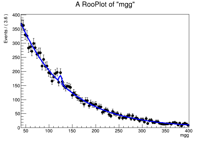
Visualize result
In [7]:
TCanvas* c1 = new TCanvas();
RooPlot* frame = w.var("mgg")->frame() ;
data->plotOn(frame) ;
When plotting an extended pdf you can choose to follow intrinsic prediction for the event count, rather than normalizing the plot to the observed data
To do so request a normalization scale factor 1.0 w.r.t the intrinsic expecation
In [8]:
w.pdf("model")->plotOn(frame,RooFit::Normalization(1.0,RooAbsReal::RelativeExpected)) ;
You can also highlight components of the fit as follows
In [9]:
w.pdf("model")->plotOn(frame,RooFit::Normalization(1.0,RooAbsReal::RelativeExpected),RooFit::Components("bkg"),RooFit::LineStyle(kDashed)) ;
frame->Draw() ;
c1->Draw() ;
[#1] INFO:Plotting -- RooAbsPdf::plotOn(model) directly selected PDF components: (bkg)
[#1] INFO:Plotting -- RooAbsPdf::plotOn(model) indirectly selected PDF components: ()
Now save the workspace with the data a modelconfig so that you can use RooStats to extract limits
Save the generated data as the ‘observed data’
In [10]:
w.import(*data,RooFit::Rename("observed_data")) ;
[#1] INFO:ObjectHandling -- RooWorkspace::import(w) importing dataset modelData
[#1] INFO:ObjectHandling -- RooWorkSpace::import(w) changing name of dataset from  modelData to observed_data
Create an empty ModelConfig
In [11]:
RooStats::ModelConfig mc("ModelConfig",&w);
Define the pdf, the parameter of interest and the observables
In [12]:
mc.SetPdf(*w.pdf("model"));
mc.SetParametersOfInterest(*w.var("mu"));
//mc.SetNuisanceParameters(RooArgSet(*w.var("mean"),*w.var("width"),*w.var("alpha")));
mc.SetNuisanceParameters(*w.var("alpha"));
mc.SetObservables(*w.var("mgg"));
Define the current value mu (1) as an hypothesis
In [13]:
w.var("mu")->setVal(1) ;
mc.SetSnapshot(*w.var("mu"));

mc.Print();
=== Using the following for ModelConfig ===
Observables:             RooArgSet:: = (mgg)
Parameters of Interest:  RooArgSet:: = (mu)
Nuisance Parameters:     RooArgSet:: = (alpha)
PDF:                     RooAddPdf::model[ S * sig + Bnom * bkg ] = 0.110271
Snapshot:
  1) 0x7f1a20b9fa80 RooRealVar:: mu = 1 +/- 0.459294  L(-3 - 6)  "mu"
import model into the workspace and save to file
In [14]:
w.import(mc);

w.writeToFile("model.root") ;