Statistical Tests
simple hypotheses for counting data
“What do we mean with probabilities?
The central concept in all statistic inference is the probability model, which assigns a probability to each possible outcome of an experiment. A well known and simple example in particle physics is the Poisson model, describing the outcome of a counting experiment,
defining the probability for an observation of \(N\) counts for a random process measured in a fixed time interval, where \(\mu\) events are expected on average. Poisson distributions describe a multitude of physics processes including radiactive decay and any particle physics counting experiment that analyses data taken in a fixed time interval. As the Poisson describes the distribution of possible outcomes of counting analysis with any type of event selection, independent on the complexity of the selection, it is by far the most common statistical model in particle physics. Given an expected event count \(\mu\) [1] the Poisson distribution fully specifies the probability of each possible outcome of a counting experiment.
A counting experiment example
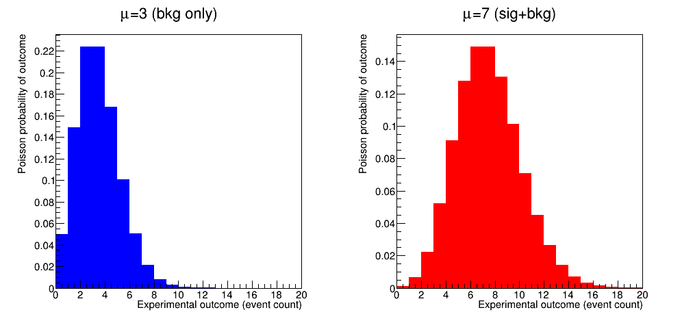
For a given hypothetical physics measurement in which, on average, 3 background events and 4 signal events are expected, Figure shows the Poisson probability distributions for the background-only hypothesis (\(\mu=3\)) and the signal-plus-background hypothesis (\(\mu=7\)). Note that the probabilities assigned by each Poisson model are strictly speaking conditional on the assumed hypothesis: suppose we observe 7 counts in our experiment, then the probability for that outcome depends on the assumed hypothesis (background-only, or signal-plus-background).
The probability of the observed data under a given hypothesis, \(P({\rm data}|H)\) as shown above, is called the Likelihood and conventionally denoted with the symbol \(\mathcal{L}\). The observation \(N=7\) is thus more likely under the \(S+B\) hypothesis than under the \(B\) hypothesis. But is this what we want to know? Or would we rather know \(P(H_{i}|N=7)\), the probability of each hypothesis given the observation of 7 counts? It turns out we don’t have enough information to calculate \(P(H_{i}|N=7)\) from \(L(N=7|H_{i})\). The relation between probabilities with inverted conditionalities is given by Bayes theorem
Thus we need to know the probabilities \(P(H)\) and \(P({\rm data})\) to be able to calculate \(P(H_{i}|N=7)\) from \(L(N=7|H_{i})\). Here, \(P({\rm data})\) is the probability of the data under any hypothesis. If only two hypotheses are considered, as is done here, then \(P({\rm data})\) can be expressed as
applying to law of total probability. Inserting Eq.tprob in Eq.bayes1 gives
where \(i\) can be \(B\) or \(S+B\). To be able to answer the question on what the value of \(P(H_{i}|N=7)\) is, the question of what the probabilities \(P(H_i)\) are then remains: these are the probabilities assigned to either hypothesis prior to the experiment. These prior probabilities can be based on earlier measurements, or can generically be considered to be a prior belief in the theory. Suppose our prior belief in \(H_{S+B}\) and \(H_{B}\) is equal, i.e. \(P(H_{S+B})=P(H_{B})=0.5\), we can then calculate
Thus the observation \(N=7\) strengthens the belief in the \(H_{S+B}\) hypothesis from 0.50 to 0.87, at the expense of the belief in the \(H_{B}\) hypothesis, which is reduced to 0.13.
The interpretation of probabilities
In the discussion so far probabilities assigned to experimental outcomes and to theories have both been used, even though they are conceptually different. Probabilities of observed data can always be interpreted as the fraction of outcome in repeated future experiment, i.e. \(P(N=7|H_{S+B})=0.14\) is interpreted as “in 14% of all future repeated identical experiments we expect the outcome \(N=7\). This frequency-based interpretation of probability is the basis of the classical, or frequentist school of statistics. In the frequentist framework no probabilities can be assigned to theories as there is no concept of repetition for hypotheses. The Bayesian school of statistics on the other hand defines probabilities as a degree of belief, that can also be assigned to hypotheses. As the Bayesian definition of probability no rule-based definition as the frequentist notion does, the probabilities are inherently subjective, although there is large effort in the statistical community to define rule-based prior probabilities that aim to reduce subjective aspects of Bayesian inference.
The different notions of probability are reflected in the type of statements that are made in statistical inference. In the frequentist framework constants of natures are fixed (the Higgs boson either exists or it doesn’t), and no probabilities can be assigned to these. Frequentist statements are thus restricted to probabilities on data. In the Bayesian framework probabilities are assigned to constants of nature (the top quark mass has a 68% probability to be in the interval \(172.2 \pm 0.7\) GeV). As the ultimate goal of any experiment is to make statements on a theory, the choice of the Bayesian of Frequentist framework is largely on the decision at what level to communicate the (numeric) experimental results that form the basis of decision. In the frequentist paradigm probabilities of data are communicated with an objective definition, that can be used for further (subjective) decision making in a later stafe. In the Bayesian paradigm, prior probabilities are inevitable included in the communicated numeric result, and thus communicate a message that contains more (subjective) information than the pure result of the experiment, and give more guidance on the conclusions that should be drawn from the data.
In this context it is intructive to compare the formulation of evidence for discovery of a new particle in both frameworks. In the Bayesian framework evidence for a hypothesis is case as an odds ratio. The ratio of probabilities prior to the experiment defines the prior odds ratio
The posterior odds ratio is defined as the ratio of posterior probabilities, calculated using Eq ref bayes1, where the denominators cancel in the ratio,
The posterior odds ratio can be factorized as the prior odds ratio multiplied with the so-called Bayes factor that contains the experimental information, as shown above. For example, for equal prior odds and an observation \(L({\rm data}|H_{B})=10^{-7}\) and \(L({\rm data}|H_{S+B})=0.5\) the posterior odds ratio becomes 2.000.000:1 in favor of the S+B hypothesis.
In the frequentist paradigm we restrict ourselves to a statement the probability of the observed data, \(L({\rm data}|H_{B})=10^{-7}\) and \(L({\rm data}|H_{S+B})=0.5\) and no notion of prior probabilities on the hypotheses exists, and it is these numbers that constitute final numeric statement. Traditionally, the conclusion that hypothesis B is ruled out is based on the observation of a very small value of \(P({\rm data}|H_{B})\) and a not-so-small value of \(P({\rm data}|H_{S+B})\), and that therefore the signal in the S+B hypothesis is considered ‘discovered’. No formal rules exist to define a discovery threshold, but probality of less than \(2.87 \cdot 10^{-7}\), corresponding to the probability of a \(\ge 5 \sigma\) fluctuation of a unit Gaussian, is traditional considered the threshold for discovery.
In the discussion of discovery threshold one should keep in mind that the probabilistic statement is often only one of the ingredients in the declaration of a discovery: For example for the Higgs boson discovery a \(5 \sigma\) observation was accepted as sufficient evidence, given that the underlying theory was well accepted, whereas much stronger statistical evidence for superluminuous neutrinos was rejected (in retrospect rightfully so), on the basis that they underlying theory was highly implausible, and that a mistake in the experimental analysis was more plausible.
The choice for a Bayesian or Frequentist interpretation of probabilities has a history of long-running discussion in particle physics. Nowadays most particle physics results are reported in the frequentist paradigm, whereas most other science displines use the Bayesian framework. The bulk of this lecture will focus on the construction of likelihood models, which form the basis of both methods. In the discussion of statistical inference methods frequentist methods are discussed in most detail, with the motivation that these are most relevent for todays particle physics students, while highlighting salient differences with Bayesian techniques when applicable.
| [1] | which of course will depend on details of the event selection criteria |
simple hypotheses for distributions
“p-values”
Most particle physics analyses are not simple counting experiments, but study one or more observable distributions that allow to discriminate signal and background.
Probability models for distributions
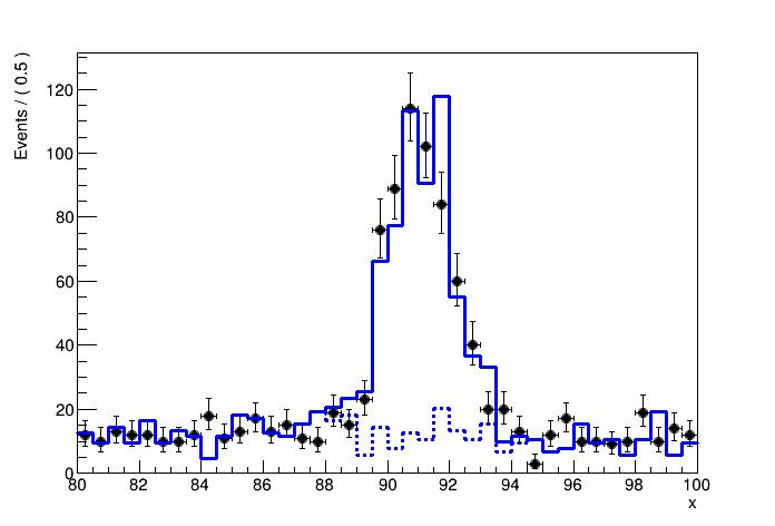
To deal with distribution in statistic inferences, we must first construct a probability model for distributions. In some cases, the distributions for observable quantities can be derived from the physics theory from first principles, resulting in analytically formulated distributions. In most cases in todays experiments, and in particular at the LHC, predicted distributions for observable quantities are derived from a chain of physics and detector simulations. The output of such simulations is histogram of simulated in events in the observable quantity. An example of such an MC simulation prodiction for a fictious signal and background process is shown in Figures binnedPdf.
While the histograms with simulated signal and background events effectively describe a distribution, the statistical model for such a binned distribution is effectively a series of counting experiments that can be described with a Poisson distribution for each bin
where \(\tilde{b}_i\) and \(\tilde{s}_i\) are the predicted event counts for the background and signal process in bin \(i\) respectively.
Statistical inferences with probability models for distributions
How does the fact that observation is a distribution change statistical inference? In the Bayesian paradigm, the likelihoods of Eq ref La, ref Lb can simply be plugged into Eq ref bayes2, and all further statistical inference procedures are unchanged. The frequentist calculation of \(L(\vec{N}|H_{B})\) also remains unchanged, but raises the question if the probability of the observed data is still relevant when drawing conclusions on the hypotheses considered: \(L(\vec{N}|H_{B})\) is the probability to observe the precise (binned) distribution of data that was recorded. That is usually not what we are interested in. We are interested in the probability to observe this, or any ‘similar’ dataset, e.g. with a few statistical fluctuations w.r.t to the observed data that correspond to the same signal event count, or larger. To introduce a precise, unambiguous notion, of what ‘more signal’ (or more generically ‘more extreme’ in any sense) means in the context of statistical inference, a test statistic is introduced in frequentist inference.
Ordering results by extremity, test statistics and p-values
A test statistic is, generically speaking, any function \(T(x)\) of the observable data \(x\). The goal of a test statistic is that it orders all possible observations \(x\) by extremity: \(T(x)>T(x')\) means that the observation \(x\) is more extreme than observation \(x'\). For example, for a Poisson counting experiment, the trivial choice \(T(x)=x\) defines a useful test statistic that orders all possible observation by extremity as more observed events means more signal for a counting experiment. With the notion of ordering possible outcomes by extremity, comes the concept of \(p\)-values. A \(p\)-value is the probability to obtain the observed data, or more extreme, in future repeated experiments. For example, for the probability to observe 7 counts or more for a Poisson counting experiment with the background hypothesis of the previous example (\(\mu=3\)) is
A \(p\)-value is always specific to the hypothesis under which it is evaluated. When no specification is given, it usually refers the to null-hypothesis, which is for discovery-style analyses the background-only hypothesis.
When the observed data is a distribution, rather than event count, the choice of \(T(x)=x\) will no longer work. We need a test statisticl to quantity if one (multi-dimensional) histogram of observed data \(\vec{N}\) is more extreme than another one. A useful test statistic for distribution is the likelihood ratio test statistic
One can intuitively see that \(\lambda(\vec{N})\) orders datasets according to signal extremity: For a dataset \(N_S\) that is very signal-like \(L(\vec{N_S}|H_{S+B})\) will be large, since the data is probable under this hypothesis, and \(\vec{N_S}|H_{B})\) will be small, since the data is improbable under this hypothesis, hence the ratio will be large. Conversely for a dataset \(N_B\) that is very background-like \(L(\vec{N_B}|H_{S+B})\) will be small, since the data is probable under this hypothesis, and \(L({\vec{N_B}}|H_{B})\) will be large, since the data is improbable under this hypothesis, hence the ratio will be large.
With a likelihood-ratio test statistic, frequentist \(p\)-values can be calculated for observable data distributions or arbitrary complexity as the test statistic \(T(\vec{x})\) maps any dataset \(x\) into a single number \(T(x)\), reducing the \(p\)-value calculation to an integral over the expected test statistic distribution under a given hypothesis
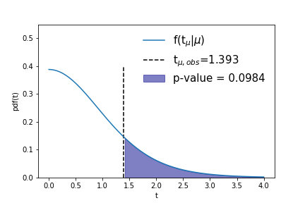
where \(f(T|H_{i})\) is the expected distribution of values of the test statistic \(T\) under the hypothesis \(H_i\). Note that the Poisson example of Eq ref poisT follows from the general form of Eq ref Tdist with the choice \(T(N)=N\) and \(H_i = {\rm Poisson}(\mu=3)\), where integration was replaced with a summation because of the integer nature \(T(N)=N\). Figure ref tsdist illustrates the concept of the distribution of the test statistic and its relation to the definition of the p-value.
![]()
A practical complication in the calculation of \(p\)-values for distribution is that, unlike the Poisson example with \(T(x)=x\) where distribution of \(T(x)\) is known because it simply the Poisson distribution of \(x\) itself, the distribution \(f(T|H_i)\) is generally not known. A simple, but but computionally expensive solution is the estimate the distribution \(f(T|H_i)\) from toy Monte Carlo simulation: a histogram of the \(T(x)\) values from ensemble of toy datasets \(x\) drawn from the hypothesis \(H_i\) will approximate the distribution \(f(T|H_i)\). For certain choices of \(T(x)\) analytical distributions are known under asymptotic conditions, and will be discussed in Section ref composite
While not discussed further in these lecture notes, for situations where analytical prescriptions are known for the distribution of observable quantities \(x\), the concept of a probability model can be extended into the concept of a probability density model \(f(x)\) where \(\int f(x) dx \equiv 1\) and the definite integral \(\int_a^b f(x) dx\) represents the probability to observe an event in the observable range \(a<x<b\). All of the statistical inference techniques discussion in this section can be identically executed using such probability density function instead of probability models.
Hypothesis tests as basis for event selection
“Optimal event selection and machine learning”
In the example Poisson model studied so far, we have focused on the statistical analysis of a counting experiment that is performed in an otherwise unspecified event selection. Designing an optimal event selection for a particular signal problem is nevertheless a core element of particle physics data analysis, and usually precedes statistical analysis of the selected event. The reason it is discussed in this lecture after an introduction on test statistics is that the theoretical basis for optimal event selection is closely connected to the likelihood ratio test statistic. In fact, with the introduction of the likelihood ratio test statistic we have already solved optimal the event selection problem for simply hypotheses: any selection defined by a lower cut on the likelihood ratio test statistic
will select on the most signal-like events in the total collection, only leaving the issue of deciding on cut the value that will define the desired purity of the selection.
The general concept of event selection relates to the statistical subject of classical hypothesis testing. In classical hypothesis testing we define two competing hypothesis, traditional called the null hypothesis \(H_0\), representing the background hypothesis in event selection, and the alternate hypothesis \(H_1\) representing the signal hypothesis in event selection. The goal of an event selection is to select as many signal events as possible, while rejecting as many background events as possible. The succes at meeting these competing goals is quantified in two measures:
- The ‘type-I’ error rate \(\alpha\), also called the size of the test. This rate represent the false positive rate, e.g. unjustly convicted suspects in trial, or background events mistakenly accepted in the signal selection.
- The ‘type-II’ error rate \(\beta\), where \(1-\beta\) is also called the power of the test. This rate represent the false negative rate, e.g mistakenly acquitted criminals or signal events mistakenly not selected in the signal region.
In general classical hypothesis testing, these goals are treated asymmetrically to construct an unambiguous optimization goal: the false positive rate \(\alpha\) is usually fixed to user-defined acceptable level (e.g. 5%), and the false negative rate \(\beta\) is then minimized. In HEP event selection problems on the other hand, no fixed value for \(\alpha\) is typically assumed, instead the optimal tradeoff between \(\alpha\) and \(\beta\) is chosen with the aid of a figure of merit that quantifies the performance of the statistical analysis of events in the signal region, such as the expected significance of the signal.
In 1932 Neyman and Pearson demonstrated that the optimal event selection for a problem with two competing hypotheses ( \(H_0\) = background and \(H_1\) = signal) the region \(W\) that minimizes the type-II error rate \(\beta\) for a given type-I error rate \(\alpha\) is defined by a contour of the likelihood ratio,
which is form very similar to the likelihood ratio test statistic \(\lambda(\vec{x})\) of Eq. ref lambda. The NP lemma also proves that \(\lambda(\vec{x})\) is an optimal test statistic, i.e. no information that distinguishes \(H_{S+B}\) from \(H_{B}\) is lost in the compactification \(\vec{x} \to T(\vec{x})\).
Even though Eq. ref NPlemma provides the optimal event selection for a signal and background events characterized by hypotheses \(H_1\) and \(H_0\), it is not always a practical criteria: it requires that the probabilities \(L(x|H_1)\) and \(L(x|H_0)\) are calculable for any \(x\). In practice the only information available on \(H_0\) and \(H_1\) is an ensemble of simulated events \(x\) drawn from each hypothesis. Except for low dimensions of \(x\), where a histogram in \(x\) can be populated for the full phase space, the ensembles of simulated events do not allow to calculate the probabilities \(L(x|H_1)\) and \(L(x|H_0)\) that are required to use Eq. NPlemma.
Instead a different strategy can be followed that is aimed at approximating the optimal decision boundary with an Ansatz function with parameters that can be “machine learned”, or otherwise inferred from training data.
Composite hypotheses (with parameters) for distributions
“Confidence intervals and maximum likelihood”
All statistical techniques discussed so far were based on simple hypotheses in which the distribution of observables is fully specified. In other words, simple hypotheses cover situations in which there are no known uncertainties in the model that is intended to describe the data. Most practical problems in physics analysis however involve a multitude of uncertain effects, ranging from uncertain calibration constants to unknown signal cross-sections. These uncertainties are accounted for in the concept of composite hypotheses, which can have one or more parameters whose value is a priori not precisely known. To illustrate the concept of composite hypothesis we extend the Poisson counting experiment of the previous section into a composite hypothesis by introducing the signal rate as a model parameter, rather than having it as a known constant [2]
Figure ref poisson_composite shows the probability distribution for possible counting outcomes of Eq. ref poisson_sb for various assumed values of its parameter \(s\). A composite hypothesis can have any number or type of parameters. Parameters are usually distinguished in two types: “parameters of interest”, and “nuisance parameters”. A parameter of interest (POIs) is any parameter that one is ultimately interested in, e.g. the reported physics quantity of the analysis. Many analyses have a single parameter of interest, but multiple POIs can also occur, for example in a measurement of Higgs boson couplings each coupling will have its own POI. Nuisance parameters are then implicitly defined as all other model parameters that are not of interest. Typically nuisance parameter described uncertainties in detector modelling (calibration uncertainties, efficiencies) and theoretical modelling (factorization/normalization scales). We will now first consider composite hypothesis with a single parameter of interest and no nuisance parameters, returning to the issues of nuisance parameters in Section ref np. Where statements on simple hypotheses were limited to \(P(data|H)\) and \(P(H|data)\) composite hypothesis offer a new range of probabilistic statements that can be made on the model parameter (of interest):
- Parameter value and variance estimation: e.g. \(s = 4.3 \pm 0.7\)
- Confidence intervals: e.g. \(s < 7.7\) at 95% C.L.
- Bayesian credible intervals: e.g \(s < 7.6\) at 95% credibility
Parameter estimations determines for which value \(\hat{s}\) of the parameter \(s\) the observed data is most probable. A parameter variance estimate determines the variance of such a point estimate, where the variance is defined in the usual way as \(\left<s^2\right> - \left<s\right>^2\). The variance expresses how much the point estimate \(\hat{s}\) will vary in repeated identical experiments. Confidence intervals and Bayesian credible intervals convey conceptually similar information, but with different definitions and properties.
Maximum Likelihood parameter estimation
The procedure to obtain the value \(\hat{s}\) of a model parameter \(s\) for which the data is most probably is called the method of maximum likelihood. The procedure entails finding the value \(s\) for which \(L(s)\) is maximal. For a simple likelihood like that of Eq. ref poisson_sb the estimation \(s\) can be performed analytically by differentiation, for more complex likelihood expressions the estimations is performed numerically, where it is customary to find the maximum of \(-\log L(s)\) rather than the maximum of \(L(s)\) as it is numerically more stable:
The standard notation is that \(\hat{p}\) is the (maximum likelihood) estimator of parameter \(p\): it represents value of \(p\) that is obtained by running the (maximum likelihood) estimation procedure on that parameter. Figure ref poisson_shat shows the value of the negative log-likelihood \(-\log L(N=7|s)\) for the Poisson model of Eq. ref poisson_sb where \(\hat{b}=5\). Note that the \(L(N|s)\) is continuous in \(s\), even though \(N\) only takes integer values. The maximum likelihood \(\hat{s}\) is the value of \(s\) for which \(-\log L(s)\) is minimal, i.e. \(\hat{s}=2\).
Maximum likelihood estimators are commonly used because they have desirable properties: ML estimators are in general
- Consistent: you get the correct answer in the limit of infinite statistics
- Mostly unbiased: the bias is proportional to \(1/N\), which becomes small compared to the estimated uncertainty proportional to \(1/\sqrt{N}\) for moderate \(N\).
- Efficient for large :math:`N`: The actual variance of ML estimator \(s\) will not be larger than \(\left<s^2\right> - \left<s\right>^2\).
- Invariant: A transformation of parameters will not changes the answer, i.e. \((\hat{p})^2 = \widehat{p^{2}}\).
In particular, the Maximum Likelihood Efficiency theorem states that a ML estimator will be efficient and unbiased for a given composite hypothesis if an unbiased efficient estimator exists for that hypothesis (proof not discussed here).
Parameter variance and the central limit theorem
It is important to note that term “uncertainty on a parameter estimate” is not uniquely defined. Multiple procedures exist that define intervals on parameters, that may yield different results depending on the underlying distributions. One of the common procedure to define an uncertainty is to take the square-root of the variance of the parameter, defined as
For Gaussian distributions an \(1 \sigma\) interval defined by \(\sqrt{V}\) will contain 68% of the distribution. For other distributions this fraction may be different, nevertheless the variance is a well-defined distribution for almost any distribution [3]. In practice most distributions that do not suffer from very low statistics are approximately Gaussian due to the Central Limit Theorem CLT) which states that the sum of \(N\) independent measurement \(x_i\), each taken from a distribution of mean \(m_i\) and a variance \(V_i\) has an expectation value \(\left< x \right> = \sum_i \mu_i\), a variance \(V_x = \sum_i V_i\) and becomes Gaussian in the limit of large \(N\). Figure ref clt demonstrates this property of the CLT for a sum of 2,3,12 measurements \(x_i\) , each drawn from a very non-Gaussian flat distribution, where the \(N=12\) case already results in a very Gaussian distribution. The variance \(V_p\) of a parameter estimate \(\hat{p}\) can be obtained with the Maximum Likelihood Variance estimator
The ML variance estimator is only efficient, i.e it will not estimate variance larger than the true variance, when the ML estimator of \(p\) is unbiased, which is usually the case at moderate to high statistics.
Confidence intervals
Another approach to defining intervals on parameters is the frequentist confidence intervals. The advantage of such fundamental methods is that they make no assumptions on the distribution (and are therefore useable in very low statistics cases) and return calibrated probabilistic statements, i.e. a 68% confidence interval definition does not rely on the fact that the underlying distribution is Gaussian.
The classical, or frequentist confidence intervals arrives at this calibrated and distribution-independent statement as follows. Given a probability model \(f(x|\mu)\) with a single parameter \(\mu\), the expected distribution of the observable \(x\) is mapped out for all values of \(\mu\) (see Fig ref nmconstr a). Next, an acceptance interval is defined for the distribution of \(x\). A simple and common way to define an acceptance interval is to take a 68% central interval, i.e. defined the interval such that 16% of the distribution sits on both the left and right side of the defined interval (Fig ref nmconstr b). Then these accepted regions in \(f(x|\mu)\) are connected for all values \(\mu\) ((Fig ref nmconstr c). This region in \(f(x|\mu)\)-vs-mu space is called the confidence belt. To defined a confidence interval on \(\mu\), a line at the observed value \(x_{obs}\) is intersected with the confidence belt to obtain the interval \([\theta_{-},\theta_{+}]\). The result of this procedure, called the Neyman Construction, is that the true value of \(\theta\), guaranteed to be contained in 68% of repeated measurements of this type, without assumptions on the distribution \(f(x|\mu)\). Confidence intervals can also take different shapes. For example, when instead of a 68% central interval, a 95% lower interval is chosen as acceptance region in \(f(x|\mu)\), the resulting confidence interval on \(\theta\) will be a 95% upper limit. Confidence intervals thus provide great flexibility in the form in which results can be formulated, dependening on the ordering rule, the procedure that is chosen to define an acceptance interval on \(f(x|\mu)\).
Note that frequentist confidence intervals strictly make no probabilistic statement about the true value of \(\mu\). In the frequentist concept of probabilities the true value of \(\mu\) is fixed, but unknown, and no probability distribution can be assigned to it. Instead the interval estimation procedure is constructed such that the intervals it produces are guaranteed to contain in exactly 68% (or 95%) of the repeated identical measurements the true (but unknown) value.
Confidence intervals using likelihood ratios
The text-book case of the construction of confidence intervals as shown in Fig ref nmconstr works only for simple probability models with a single observable \(x\). To define confidence intervals on probabity models where the observable \(x\) is not a single number, but a (multi-dimensional) distribution, the likelihood ratio technique introduced earlier in Section 3.3 comes to the rescue. Instead of taking an ordering rule that defines an interval in \(f(x|\mu)\), a new ordering rule is introduced that instead defines an interval on a likelihood ratio based on \(f(x|\mu)\)
to define a confidence belt. Whereas the text-book confidence belt of Fig ref nmconstr provided an intuitive graphical illustration of the concept of acceptance intervals on \(x\) and confidence intervals in \(\mu\), a confidence belt based on a likelihood-ratio ordering rule may seem at first more obscure, but in reality isn’t. Figure ref nmconstr2 compares side-by-side the text-book confidence belt of \(f(x|\mu)\) with a LLR-based confidence belt of \(\lambda(\vec{N}|\mu)\). We observe the following differences
- The variable on the horizontal axis is \(\lambda(\vec{N}|\mu)\) instead of \(f(x|\mu)\). As \(\lambda(\vec{N}|\mu)\) is a scalar quantity regardless of the complexity of the observable \(\vec{N}\) this allows us to make this confidence belt construction for any model \(f(\vec{N}|\mu)\) of arbitrary complexity.
- The confidence belt has a different shape. Whereas the expected distribution \(f(x|\mu)\) is typically different for each value of \(\mu\), the expected distribution of \(\lambda(\vec{N}|\mu)\) typically is independent of \(\mu\). The reason for this is the asymptotic distribution of \(\lambda(\vec{N}|\mu)\) that will be discussed further in a moment. The result is though that a LLR-based confidence belt is usually a rectangular region starting at \(\lambda=0\).
- The observed quantity \(\lambda(\vec{N}|\mu)_{obs}\) depends on \(\mu\) unlike the observed quantity \(x_{obs}\) in the textbook case. The reason for this is simply the form of Eq.ref{eq:llr} that is an explicit function of \(\mu\). Asymptotically the dependence of \(\lambda(\vec{N}|\mu)\) on \(\mu\) is quadratic, as shown in the illustration.
The confidence belt construction shown in Fig ref nmconstr2, when rotated 90 degrees counterclockwise looks of course very much like an interval defined by a rise in the likelihood (ratio), as is done by MINUITS MINOS procedure, and that correspondence is exact in the limit of large statistics. This last observation brings about an important point: in the limit of large statistics, the ‘simple’ procedure of defining an interval by a rise in the likelihood ratio defines a proper frequentist confidence interval with its desirable properties: the result is independent of the distribution and the quoted (68 or 95%) confidence level is calibrated. This asymptotic correspondence of the completely general (and potentially) expensive Neyman Construction procedure with its desirable calibration properties and asymptotic and computationally light likelihood ratio interval procedure occurs when Wilks theorem is satisfied, i.e that the distribution of \(\lambda(\vec{N}|\mu)\) for data sampled under the hypothesis \(\mu\) is asymptotically distributed as a \(\chi^2\) distribution, and therefore is independent of \(\mu\). Note that this condition does not imply that the likelihood ratio as function of \(\mu\) is exactly parabolic, thus the interpretation of asymmetric MINOS error as frequentist confidence intervals is correct as long as Wilks theorem is met. When in doubt, one can check this requirement by verifying that the distribution of \(\lambda(\vec{N}|\mu)\) values from a suitable large sample of toy datasets follows the asymptotic \(\chi^2\) distribution, as is shown in Figure ref wilks.
Confidence intervals with boundaries
As frequentist confidence intervals make statements on the frequency of measured values and do not aim to interpret these measurement values as a probabilistic statement on constants of nature as a Bayesian procedure does, the occurence of intervals that (partially) cover unphysical values do not pose a problem. A classical situation of this type is the Poisson counting experiment where the observed event count is less than the expected background event count. For example, for a counting experiment with 10 expected background events and 3 expected signal events, an observation of 8 events is entirely unproblematic, although the resulting parameter estimate of -2 signal events is sometimes frowned upon. The key to interpreting such a result is to realize that -2 signal events is strictly the outcome of a measurement procedure, and is expected to occur at some frequency. If the negative fluctuation is substantial, e.g. 5 observed for 10 expected background, it can happen that the resulting interval estimate only brackets negative values for the signal count, in other words, all signal counts greater than 0 are excluded, at 95% confidence level. Also this is, strictly speaking, not a problem, as the true value is outside the quoted interval in 5% of the measurements by construction. Nevertheless, many physicists are uncomfortable quoting a result of this type as the final outcome as the result of a physics measurement.
It is possible to adjust the construction procedures of confidence intervals such that such unphysics intervals cannot occur and yet respect the essential calibration property of the Neyman construction - namely that the reported intervals are guaranteed to contain the true value in 68% or 95% of the cases. The key to accomplish this is to only modify the ordering rule, but leave the Neyman construction itself (which guarantees the calibration) unchanged. To do so the standard likelihood ratio ordering rule, encoded by
is replaced by
The ordering rule \(\tilde{t}\) changes the interpretation of observations with \(\hat{\mu}<0\). Consider the ordering rule for the no-signal hypothesis (mu=0) for an observation of \(\hat{\mu}=-2\): The traditional test statistic \(t_{\mu}\) will consider this observation to be inconsistent with the no-signal hypothesis: \(\log(L(x|0)/L(x|-2))\) will be larger than zero. At as sufficiently negative \(\hat{\mu}\), when \(t_{\mu}\) becomes larger than 0.5 for \(\mu=0\), the points \(\mu\ge 0\) will be excluded from a 68% confidence interval and once it becomes larger than 2, the points \(\mu\ge 0\) will also be excluded at 95% C.L.
The modified test statistic \(\tilde{t}_{\mu}\) will on the other hand consider any observation with \(\hat{\mu}<0\) to be maximally consistent with the no-signal hypothesis: \(\log(L(x|0)/L(x|0))\) will be exactly zero for any observation with \(\hat{\mu}<0\)! The effect of this modification on the resulting confidence belt is that \(\mu=0\) is inside the confidence interval corresponding to any observation with \(\hat{\mu}<0\) , hence no downward fluctuations w.r.t the background estimate will result in the exclusion of \(\mu=0\). In practice, small positive values of \(\mu\) will also not be excluded, hence any observation with \(\hat{\mu}<0)\) will result in a confidence interval \([0,\mu_{+}]\), with the size of the confidence interval decreasing with decreasing \(\hat{\mu}<0)\).
Observations of event counts much larger than the background estimate, on the other hand, do not trigger such special handling. Thus the observation of a very large positive event count will exclude \(\mu=0\) from the confidence interval, and result as usual in a two-side confidence interval \([\mu_{-},\mu_{+}]\), corresponding to a measurement-style result. The point where the transition from a one-sided interval of the from \([0,\mu_{+}]\) transitions into a two-sided interval \([\mu_{-},\mu_{+}]\) is automatically determined by the procedure. In the HEP literature the confidence intervals constructed with an ordering rule based on the modified likelihood ratio \(\tilde{t}_{\mu}\) is usually called the ‘modified frequentist procedure’, or Feldman-Cousins, and is considered to be a ‘unified’ procedure as the transition from upper limits to two-sided intervals is automatically determined. As for \(t_{\mu}\), asymptotic distributions for the modified test statistic \(\tilde{t}_{\mu}\) are known, and are discussed in detail in [X].
| [2] | To facilitate the distinction between symbolic constant expressions (a known background) and symbolic parameters (an unknown background) all constant symbols are marked with a tilde: i.e. \(\tilde{a}\) is constant expression, whereas \(a\) is a parameter. |
| [3] | An notable example of a distribution that has no well-defined mean or variance is the non-relativistic Breit-Wigner distribution. |
Bayesian credible intervals
The introduction of composite hypotheses in Bayesian statistics transforms Bayes theorem from an equation calculating probabilities for hypothesis, into an equation calculating probability densities for model parameters, i.e.
Statistical inference with nuisance parameters
“Fitting the background”
In all examples of this course so far, we have only considered ideal experiments, i.e. experiments that have associated systematic uncertainties originating from experimental aspects or theoretical calculations. This section will explore how to modify statistical procedures to account for the presence of parameter associated to systematic uncertainties, whose values are not perfectly known.
What are systematic uncertainties
The label systematic uncertainty strictly originates in the domain of the (physics) problem that we are trying to solve, it is not a concept in statistical modelling. In practice, a systematic uncertainty arises when there effect whose precise shape and magnitude is not know affects our measurement, hence we need to have some estimate of it. A common approach is that we aim capture the unknown effect in one or more model parameters, whose values we then consider the not perfectly known. A good example is a detector calibration uncertainty that affects an invariant mass measurement. If the assumed calibration in the statistical analysis is different from the true (but known) calibration of the detector the measurement will be off my some amount. In most cases some information is available on the unknown calibration constant, in the form of a calibration measurement with an associated uncertainty “the energy scale of reconstructed jets has a 5% uncertainty”. An example of a systematic uncertainty arising from theory is a cross-section uncertainty on a background process in a counting experiment. In both these cases the goal is propagate the effect of the uncertainty on the parameter associated with the theoretical uncertainty to the measurement of the parameter of interest. In the discussion of systematic uncertainties there are hence two distinct aspects that should be distinguished
- Identifying which are the degrees of freedom associated with the conceptual systematic uncertainty, and implement these as model parameters
- Account for the presence of these uncertain model parameters in the statistical inference.
The first aspect is a complex subject that is strongly entangled in the physics of the problem that one aims to solve and is discussed in detail in the next section, whereas the second subject is purely on statistical procedure, and is discussed in this section following a simple example likelihood featuring one or more such “nuisance parameters”.
Treatment of nuisance parameters in parameter point and variance estimation
To illustrate the concept of nuisance parameter treatment in point and variance estimation, we can construct a simple extension of the Poisson counting example introduced in Equation X33, by now considering the background that was previously assumed to exactly known, to be unknown, and measurement from a second counting experiment that only measures the backgroundfootnote{The experiment is constructed such that the background rate measurement in the control regions is three times the expected background rate in the signal region.}
The likelihood function of Eq. ref PoissonSB can be used to construct a 2-dimensional measurement of both \(s\) and \(b\) following the procedures outline in Section X, but given that we are now only interested in the signal rate \(s\) and not in the background rate \(b\), the goal is to formulate a statement on \(s\) only, while taking into account the uncertainty on \(b\). Figure ref PoissonSB2D shows the 2-dimensional likelihood function for \(L(s,b)\) for an observation of \(N_{SR}=10, N_{CR}=10\). A likelihood \(L(s)\) without nuisance parameters that assumes \(b=5\) corresponds to the slice of the plot indicated at the dashed line and will estimate \(\hat{s}=5\), where the maximum likelihood is found in that slice. A likelihood \(L(s,b)\) with \(b\) as a nuisance parameter will instead find the minimum \(\hat{b}=3.3,\hat{s}=6.7\), with the effect of the nuisance parameter ostensibly taken into account.
The effect of the nuisance parameter \(b\) on the variance estimate of \(s\) comes in through the extension of the one-dimensional variance estimator into a multidimensional covariance estimator
If the estimators of \(s\) and \(b\) are correlated, the off-diagonal elements of the matrix in Eq. ref covariance are non-zero and the variance estimates on \(s\) using \(V(s)\) and \(V(s,b)\) will differ. This difference in variance is visualized in Fig ref covsb that shows a contour of \(L(s,b)\) in the \(s,b\) plane assuming a Gaussian distribution for a scenario where the estimates of \(s,b\) are somewhat anti-correlated (left) and uncorrelated (right). The square-root of the variance estimate on \(s\) using \(V(s)\) corresponds to the distance between the intersection of the the line \(b=\hat{b}\) with the likelihood contour (red line). The square-root of the variance estimate on \(s\) using \(V(s,b)\) corresponds the size of the box that encloses the the contour. If the estimators of \(s\) and \(b\) are uncorrelated, both methods will return the same variance, reflecting that the uncertainty on \(b\) has no impact on the measurement of \(s\). If on the other had the estimators of \(s\) and \(b\) are correlated, the variance estimate from \(V(s,b)\) will always be larger than the estimate from \(V(s)\), reflecting the impact of the uncertainty on \(b\) on the measurement on \(s\).
Treatment of nuisance parameters in hypothesis testing and confidence intervals
The calculation of \(p\)-values for hypothesis testing in models with a parameter of interest \(\mu\), but without nuisance parameters is based on the distribution of the test statistic \(p_{\mu} = \int_{t_{\mu,obs}}^{\infty} f(t_{\mu}|\mu) dt_{\mu}\) where \(t_\mu\) is the test statistic (usually a likelihood ratio), \(f(t_\mu|\mu)\) is the expected distribution of that test statistic and \(t_{\mu,obs}\) is the observed value of the test statistic. With the introduction of a generic nuisance parameter \(\theta\), i.e. \(L(\mu) \to L(\mu,\theta)\) the distribution of a test statistic based on that likelihood (ratio) will generallly also depend on \(\theta\)
and hence the question now is, what value of \(\theta\) to assume in the distribution of \(t_{\mu}\)? Fundamentally, we want to reject the hypothesis \(\mu\) at \(\alpha\%\) C.L. only if \(p_{\mu}<1-\alpha\) for any value of :math:`theta`. In other words, if there is any value of \(\theta\) for which the data is compatible with hypothesis \(\mu\) we do not want to reject the hypothesis. This approach appears a priori extremely challenging both technically (performing the calculation for each possible value of \(\theta\)) also conceptually (one should really consider values of \(\theta\) that are itself excluded by other measurements), but it turns out that with a clever choice of \(t_{\mu}\) the statistical problem becomes quite tractable. The key is to replace the likelihood ratio test statistic with the profile likelihood ratio test statistic
where the symbol \(\hat{\hat{\mu}}\) represents the conditional [4] maximum likelihood estimate of \(\theta\). Note that the profile likelihood ratio test statistic \(\Lambda_{\mu}\) does explicitly not depend on the Likelihood parameter \(\theta\) as both \(\hat{\theta}\) and \(\hat{\hat{\theta}}\) are determined by the data. In the limit of large statistics the distribution of the test statistic \(f(\Lambda_{\mu}|\mu_{true},\theta_{true})\) follows a \(\chi^2\) distribution, just like the distribution of \(t_{\mu}\). This is nice for two reasons: first it allows us to reuse the formalism developed for the construction of confidence intervals based on \(t_{\mu}\) to be recycled for \(\Lambda_{\mu}\) by simply replacing the test statistic. Second it means that \(f(\Lambda_{\mu}|\mu_{true},\theta_{true})\) is asymptotically independent of the true value of both \(\mu_{true}\) and \(\theta_{true}\) so that the interval based on \(\Lambda_{\mu}\) convergence to a proper frequentist interval even in the present of nuisance parameters in the asymptotic limit.
It is instructive to compare the plain likelihood ratio \(t_{\mu}\) and profile likelihood ratio \(\Lambda_{\mu}\) for an example model: the distribution of an observable \(x\) that is described by a Gaussian signal and and order-6 Chebychev polynomial background. The corresponding likelihood function has one parameter of interest, the signal strength, and 6 nuisance parameters, the coefficients of the polynomial. Figure ref plrdemo shows the distribution of the plain likelihood ratio (blue, top) and the profile likelihood ratio (red, bottom). As the likelihood model with floating nuisance parameters is generally more consistent with the observed data for each assumed value of the signal strength (as the polynomial background can be configured to peak or dip in the signal region), the confidence interval of the profile likelihood ratio is wider than that of the plain likelihood ratio, reflecting the additional uncertainty introduced on the measurement of the signal strength by the fact that the background shape is not perfectly known.
| [4] | Where the condition is that the POI is fixed at the value \(\mu\), rather than allowed to float to the value \(\hat{\mu}\) in the minimization, as is the case in the minimization of the unconditional estimate \(\hat{\theta}\) |