Build workspace using histogram templates
Build a binned likelihood model version of the ex11 example
- construct a histogram template SH(mgg) with a prediction for the binned signal shape
- construct a histogram template BH(mgg) with a prediction for the binned background shape
- construct a probability model model(mgg) = SH(mgg) + BH(mgg)
This model can be ‘seen’ in two ways
- an extended probability model like ex11 that happen to have binned shapes, i.e.
- model(mγγ) = Nsig/Nsig+Nbkg * pdfSH(mγγ) + Nbkg/Nsig+Nbkg * pdfBH(mγγ)
- \(P(N) = N_\mathrm{sig} + N_\mathrm{bkg}\)
- where pdf_SH,pdf_BH are probability density functions that follow shape of the unit normalized histograms
- A product of Poisson counting experiments for each bin
- model(vec_N) = Product(i=0..n-1) Poisson(N_i | S_i + B_i)
- where N_i i=0…N-1 == vec_N are the observed event counts in each bin and S_i and B_i are the predicted signal and background rate in each bin
Both representations are mathematically equivalent, but expression (2) is in practice faster to calculate because it does not require a normalization calculation over pdf_SH and pdf_BH to happen. While for this very simple example it does not make a noticable difference because the normalization does not depend on any model parameters in scenarios where it does it will effectivelt double the calculation time
Construct simulation workspace to generate template histograms
In [1]:
RooWorkspace wsim("wsim") ;
RooFit v3.60 -- Developed by Wouter Verkerke and David Kirkby
                Copyright (C) 2000-2013 NIKHEF, University of California & Stanford University
                All rights reserved, please read http://roofit.sourceforge.net/license.txt
Generate two distributions, exponential distribution for the background, Gaussian distribution for the signal
In [2]:
wsim.factory("Exponential::bkg(mgg[40,400],alpha[-0.01,-10,0])") ;
wsim.factory("Gaussian::sig(mgg,mean[125,80,400],width[3,1,10])") ;

RooDataHist* hist_sig = wsim.pdf("sig")->generateBinned(*wsim.var("mgg"),50) ;
RooDataHist* hist_bkg = wsim.pdf("bkg")->generateBinned(*wsim.var("mgg"),10000) ;
Mock data distribution with mu=1.5
In [3]:
wsim.factory("expr::S('mu*Snom',mu[1.5],Snom[50])") ;
wsim.factory("SUM::model(S*sig,Bnom[10000]*bkg)") ;
Given that the sum is an extended model, no speficiation of the event count is needed
In [4]:
RooDataHist* hist_data = wsim.pdf("model")->generateBinned(*wsim.var("mgg")) ;
Set up binned likelihood model
In [5]:
RooWorkspace w("w") ;
First Import template and mock data histograms
In [6]:
w.import(*hist_sig,RooFit::Rename("template_sig")) ;
w.import(*hist_bkg,RooFit::Rename("template_bkg")) ;
w.import(*hist_data,RooFit::Rename("observed_data")) ;
[#1] INFO:ObjectHandling -- RooWorkspace::import(w) importing dataset genData
[#1] INFO:ObjectHandling -- RooWorkSpace::import(w) changing name of dataset from  genData to template_sig
[#1] INFO:ObjectHandling -- RooWorkspace::import(w) importing RooRealVar::mgg
[#1] INFO:ObjectHandling -- RooWorkspace::import(w) importing dataset genData
[#1] INFO:ObjectHandling -- RooWorkSpace::import(w) changing name of dataset from  genData to template_bkg
[#1] INFO:ObjectHandling -- RooWorkspace::import(w) importing dataset genData
[#1] INFO:ObjectHandling -- RooWorkSpace::import(w) changing name of dataset from  genData to observed_data
Now build signal and background models
Note that we build functions here and not pdfs
In [7]:
w.factory("HistFunc::sig(mgg,template_sig)") ;
w.factory("HistFunc::bkg(mgg,template_bkg)") ;
[#1] INFO:ObjectHandling -- RooWorkspace::import(w) importing dataset template_sig
[#1] INFO:ObjectHandling -- RooWorkspace::import(w) importing dataset template_bkg
Also not that we don’t need to declare mgg here, its definition was imported when we imported the histograms
Now construct a ‘amplitude sum’ probability model, defined asa
scaling the predictions of the template histograms. If the template histograms encode the nominal event yield, one expects both coefficients to fit to 1 if the data matches the prediction
NOTE: If the bin width is not equal to one then the event count of a histogram is not identical to the integral over a histogram. In RooFit the **integral* over the histogram is taken as the yield prediction, whereas one usually, interprets the histogram event count as the prediction. The simplest way to correct for this is to multiply \(c_\mathrm{i}\) with a constant which is 1/binwidth*
In this case we choose \(c_\mathrm{sig} = \mu\) (as usual) and introduce a Bscale as a nuisance parameter that can freely scale the background
In [8]:
w.factory("binw[0.277]") ; // == 1/(400-30)
w.factory("expr::S('mu*binw',mu[1,-1,6],binw[0.277])") ;
w.factory("expr::B('Bscale*binw',Bscale[0,6],binw)") ;
w.factory("ASUM::model(S*sig,B*bkg)") ;
[#1] INFO:ObjectHandling -- RooWorkSpace::import(w) Recycling existing object binw created with identical factory specification
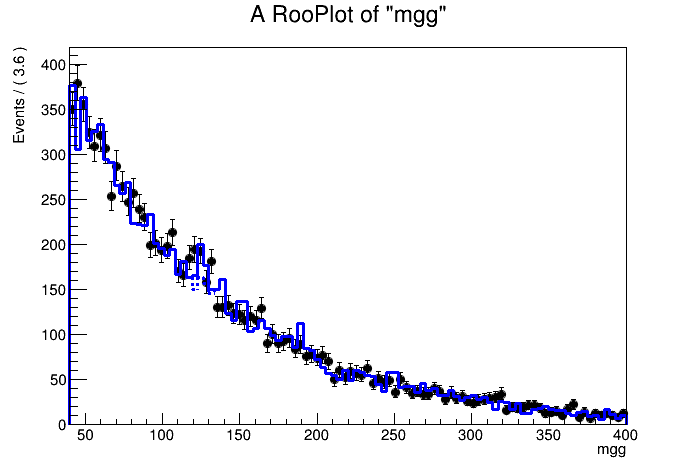
Fit the binned probability model to the binned data
In [9]:
w.pdf("model")->fitTo(*hist_data) ;
TCanvas* c1 = new TCanvas();
RooPlot* frame = w.var("mgg")->frame() ;
hist_data->plotOn(frame) ;
w.pdf("model")->plotOn(frame) ;
w.pdf("model")->plotOn(frame,RooFit::Components("bkg"),RooFit::LineStyle(kDashed)) ;
frame->Draw() ;
c1->Draw();
[#1] INFO:Minization -- p.d.f. provides expected number of events, including extended term in likelihood.
[#1] INFO:Minization -- createNLL: caching constraint set under name CONSTR_OF_PDF_model_FOR_OBS_mgg with 0 entries
[#1] INFO:Minization -- RooMinimizer::optimizeConst: activating const optimization
[#1] INFO:Minization --  The following expressions have been identified as constant and will be precalculated and cached: (sig,bkg)
 **********
 **    1 **SET PRINT           1
 **********
 **********
 **    2 **SET NOGRAD
 **********
 PARAMETER DEFINITIONS:
    NO.   NAME         VALUE      STEP SIZE      LIMITS
     1 Bscale       3.00000e+00  6.00000e-01    0.00000e+00  6.00000e+00
     2 mu           1.00000e+00  7.00000e-01   -1.00000e+00  6.00000e+00
 **********
 **    3 **SET ERR         0.5
 **********
 **********
 **    4 **SET PRINT           1
 **********
 **********
 **    5 **SET STR           1
 **********
 NOW USING STRATEGY  1: TRY TO BALANCE SPEED AGAINST RELIABILITY
 **********
 **    6 **MIGRAD        1000           1
 **********
 FIRST CALL TO USER FUNCTION AT NEW START POINT, WITH IFLAG=4.
 START MIGRAD MINIMIZATION.  STRATEGY  1.  CONVERGENCE WHEN EDM .LT. 1.00e-03
 FCN=-18731 FROM MIGRAD    STATUS=INITIATE        6 CALLS           7 TOTAL
                     EDM= unknown      STRATEGY= 1      NO ERROR MATRIX
  EXT PARAMETER               CURRENT GUESS       STEP         FIRST
  NO.   NAME      VALUE            ERROR          SIZE      DERIVATIVE
   1  Bscale       3.00000e+00   6.00000e-01   2.01358e-01   1.98597e+04
   2  mu           1.00000e+00   7.00000e-01   2.24553e-01   9.86124e+01
                               ERR DEF= 0.5
 MIGRAD MINIMIZATION HAS CONVERGED.
 MIGRAD WILL VERIFY CONVERGENCE AND ERROR MATRIX.
 COVARIANCE MATRIX CALCULATED SUCCESSFULLY
 FCN=-27643.4 FROM MIGRAD    STATUS=CONVERGED      63 CALLS          64 TOTAL
                     EDM=1.90326e-05    STRATEGY= 1      ERROR MATRIX ACCURATE
  EXT PARAMETER                                   STEP         FIRST
  NO.   NAME      VALUE            ERROR          SIZE      DERIVATIVE
   1  Bscale       1.00258e+00   1.02810e-02   5.15767e-04  -9.00358e-01
   2  mu           1.54130e+00   4.86712e-01   1.62486e-02  -1.71092e-02
                               ERR DEF= 0.5
 EXTERNAL ERROR MATRIX.    NDIM=  25    NPAR=  2    ERR DEF=0.5
  1.057e-04 -1.035e-03
 -1.035e-03  2.386e-01
 PARAMETER  CORRELATION COEFFICIENTS
       NO.  GLOBAL      1      2
        1  0.20612   1.000 -0.206
        2  0.20612  -0.206  1.000
 **********
 **    7 **SET ERR         0.5
 **********
 **********
 **    8 **SET PRINT           1
 **********
 **********
 **    9 **HESSE        1000
 **********
 COVARIANCE MATRIX CALCULATED SUCCESSFULLY
 FCN=-27643.4 FROM HESSE     STATUS=OK             10 CALLS          74 TOTAL
                     EDM=1.90282e-05    STRATEGY= 1      ERROR MATRIX ACCURATE
  EXT PARAMETER                                INTERNAL      INTERNAL
  NO.   NAME      VALUE            ERROR       STEP SIZE       VALUE
   1  Bscale       1.00258e+00   1.02822e-02   1.03153e-04  -7.28574e-01
   2  mu           1.54130e+00   4.86745e-01   3.24972e-03  -2.77461e-01
                               ERR DEF= 0.5
 EXTERNAL ERROR MATRIX.    NDIM=  25    NPAR=  2    ERR DEF=0.5
  1.057e-04 -1.038e-03
 -1.038e-03  2.386e-01
 PARAMETER  CORRELATION COEFFICIENTS
       NO.  GLOBAL      1      2
        1  0.20664   1.000 -0.207
        2  0.20664  -0.207  1.000
[#1] INFO:Minization -- RooMinimizer::optimizeConst: deactivating const optimization
[#1] INFO:Plotting -- RooAbsPdf::plotOn(model) directly selected PDF components: (bkg)
[#1] INFO:Plotting -- RooAbsPdf::plotOn(model) indirectly selected PDF components: ()
Now save the workspace with the data a modelconfig so that you can use RooStats to extract limits
Create an empty ModelConfig
In [10]:
RooStats::ModelConfig mc("ModelConfig",&w);
Define the pdf, the parameter of interest and the observables
In [11]:
mc.SetPdf(*w.pdf("model"));
mc.SetParametersOfInterest(*w.var("mu"));
//mc.SetNuisanceParameters(RooArgSet(*w.var("mean"),*w.var("width"),*w.var("alpha")));
mc.SetNuisanceParameters(*w.var("Bscale"));
mc.SetObservables(*w.var("mgg"));
Define the current value \(\mu=1\) as an hypothesis
In [12]:
w.var("mu")->setVal(1) ;
mc.SetSnapshot(*w.var("mu"));

mc.Print();
=== Using the following for ModelConfig ===
Observables:             RooArgSet:: = (mgg)
Parameters of Interest:  RooArgSet:: = (mu)
Nuisance Parameters:     RooArgSet:: = (Bscale)
PDF:                     RooRealSumPdf::model[ S * sig + B * bkg ] = 2.77715
Snapshot:
  1) 0x7fe4dca0cd80 RooRealVar:: mu = 1 +/- 0.486745  L(-1 - 6)  "mu"
import model in the workspace
In [13]:
w.import(mc);

w.writeToFile("model.root") ;